Multiple Imputation

1 Preamble

1.1 Install Libraries

Code

#install.packages("remotes")
#remotes::install_github("DevPsyLab/petersenlab")

1.2 Load Libraries

Code

library("tidyverse")
library("psych")
library("mice")
library("micemd")
library("miceadds")
library("mitml")
library("Amelia")
library("jomo")
library("parallelly")
library("future")
library("furrr")
library("nlme")
library("lme4")
library("broom.mixed")
library("MplusAutomation")

1.3 Data

Code

data(Oxboys, package = "nlme")

Oxboys_addNA <- data.frame(Oxboys)
Oxboys_addNA <- Oxboys_addNA %>% 
  rename(id = Subject)

Oxboys_addNA$id <- as.integer(Oxboys_addNA$id)
Oxboys_addNA$Occasion <- as.integer(Oxboys_addNA$Occasion)

set.seed(52242)
Oxboys_addNA[sample(1:nrow(Oxboys_addNA), 25), "height"] <- NA

dataToImpute <- Oxboys_addNA

2 Types of Missingness

Missing Completely at Random (MCAR)
- the probability of being missing is the same for all cases
- missingness is not related to variables in the model
(Conditionally) Missing at Random (MAR)
- missingness is related to variables in the model, but once we condition on the variables in the model, the missingness is haphazard
- the unobserved values do not play a role
Missing Not at Random (MNAR)
- missingness is related to variables that are not in the model (i.e., for reasons that are unknown)
- unobserved variables carry information about whether a case will have missing data

3 Approaches to Handle Missing Data

3.1 For MCAR/MAR Missingness

Full Information Maximum Likelihood (FIML)
Multiple Imputation

3.2 For MNAR Missingness

https://stefvanbuuren.name/fimd/sec-nonignorable.html (archived at https://perma.cc/N7WW-HDZF)

https://cran.r-project.org/web/packages/missingHE/vignettes/Fitting_MNAR_models_in_missingHE.html (archived at https://perma.cc/9X25-5D8G)

find more data about the causes for the missingness
sensitivity analyses (what-if analyses) to see how sensitive the results are under various scenarios
- https://stefvanbuuren.name/fimd/sec-MCAR.html (archived at https://perma.cc/9KM9-3NX3)
selection models
- simultaneously estimate the focal model and a missingness model, where the missingness model has the missing data indicator as a dependent variable, as predicted by the original dependent variable, the original predictors, and any additional covariates etc.
- if the missingness model is approximately correct, the focal model adjusts in way that removes nonresponse bias
- similar to a mediation process
  - X → Y
  - Y → missingness
  - X → missingness
- https://quantitudepod.org/s4e08-craig-enders/ (archived at https://perma.cc/FY9L-L3F7)
pattern-mixture models
- missing data indicator is a predictor variable
- similar to a moderation process; subgroups of cases have different parameter estimates

4 Approaches to Multiple Imputation

multiple imputation by joint modeling
- assumes that the variables in follow a joint distribution, e.g.:
  - multivariate normal (i.e., multivariate normal imputation)
- R packages:
  - jomo
  - pan
  - Amelia
  - Mplus
multiple imputation by chained equations
- aka:
  - fully conditional specification multiple imputation
  - sequential regression multiple imputation
- R packages:
  - mice
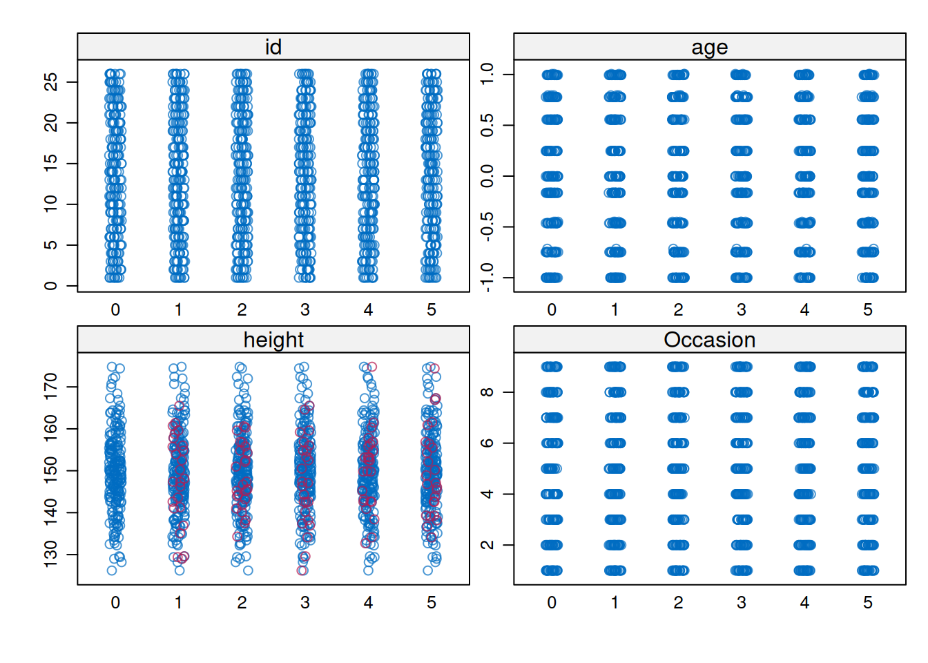
    - predictive mean matching (?mice::mice.impute.pmm) can be useful to obtain bounded imputations for non-normally distributed variables

5 Describe Missing Data

Code

describe(dataToImpute)

Code

md.pattern(dataToImpute, rotate.names = TRUE)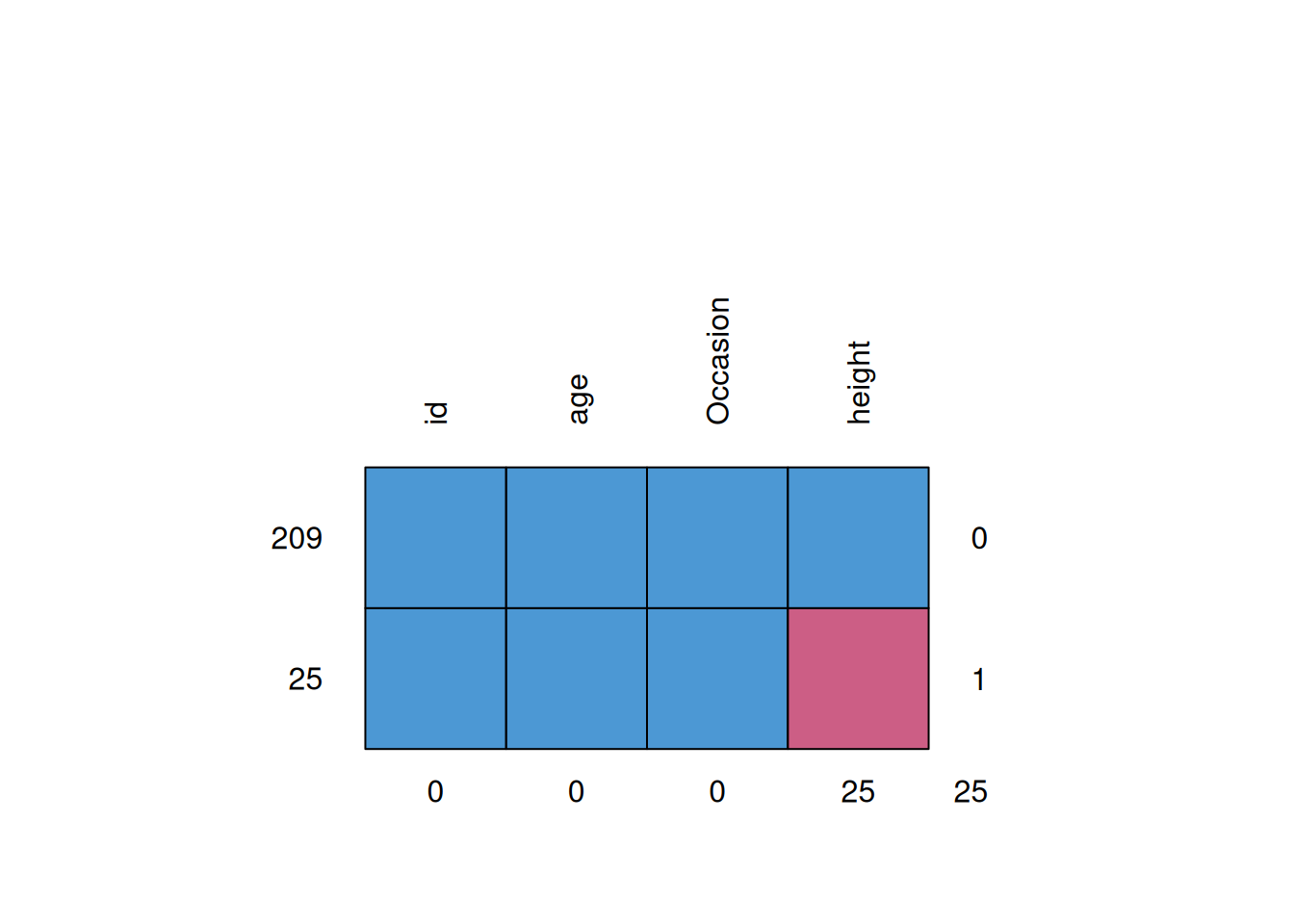

    id age Occasion height   
209  1   1        1      1  0
25   1   1        1      0  1
     0   0        0     25 25

6 Pre-Imputation Setup

6.1 Specify Variables to Impute

Code

varsToImpute <- c("height")
Y <- varsToImpute

6.2 Specify Number of Imputations

Code

numImputations <- 5 # generally use 100 imputations; this example uses 5 for speed

6.3 Detect Cores

Code

numCores <- parallelly::availableCores() - 1

7 Multilevel Multiple Imputation

7.1 Three-Level and Cross-Classified Data

https://simongrund1.github.io/posts/multiple-imputation-for-three-level-and-cross-classified-data/ (archived at https://perma.cc/N4PP-A3V6)

7.2 Methods

7.2.1 `mice`

7.2.1.1 Types

7.2.1.1.1 Continuous Outcomes

https://stefvanbuuren.name/fimd/sec-multioutcome.html#methods (archived at https://perma.cc/8CDA-TS3K)

Code

?mice::mice.impute.2l.norm
?mice::mice.impute.2l.pan
?mice::mice.impute.2l.lmer
?miceadds::mice.impute.2l.pmm
?miceadds::mice.impute.2l.contextual.pmm
?miceadds::mice.impute.2l.continuous
?micemd::mice.impute.2l.2stage.norm
?micemd::mice.impute.2l.2stage.pmm
?micemd::mice.impute.2l.glm.norm
?micemd::mice.impute.2l.jomo

7.2.1.1.2 Binary Outcomes

https://stefvanbuuren.name/fimd/sec-catoutcome.html#methods-1 (archived at https://perma.cc/5QHF-YRP6)

Code

?mice::mice.impute.2l.bin
?miceadds::mice.impute.2l.binary
?miceadds::mice.impute.2l.pmm
?miceadds::mice.impute.2l.contextual.pmm
?micemd::mice.impute.2l.2stage.bin
?micemd::mice.impute.2l.glm.bin

7.2.1.1.3 Ordinal Outcomes

https://stefvanbuuren.name/fimd/sec-multioutcome.html#methods (archived at https://perma.cc/8CDA-TS3K)

Code

?miceadds::mice.impute.2l.pmm
?miceadds::mice.impute.2l.contextual.pmm
?micemd::mice.impute.2l.2stage.pmm

7.2.1.1.4 Count Outcomes

https://stefvanbuuren.name/fimd/sec-catoutcome.html#methods-1 (archived at https://perma.cc/5QHF-YRP6)

Code

?micemd::mice.impute.2l.2stage.pois
?micemd::mice.impute.2l.glm.pois
?countimp::mice.impute.2l.poisson
?countimp::mice.impute.2l.nb2
?countimp::mice.impute.2l.zihnb

7.2.1.2 Specifying the Imputation Method

Code

meth <- make.method(dataToImpute)
meth[1:length(meth)] <- ""
meth[Y] <- "2l.pmm" # specify the imputation method here; this can differ by outcome variable

7.2.1.3 Specifying the Predictor Matrix

A predictor matrix is a matrix of values, where:

columns with non-zero values are predictors of the variable specified in the given row
the diagonal of the predictor matrix should be zero because a variable cannot predict itself

The values are:

NOT a predictor of the outcome: 0
cluster variable: -2
fixed effect of predictor: 1
fixed effect and random effect of predictor: 2
include cluster mean of predictor in addition to fixed effect of predictor: 3
include cluster mean of predictor in addition to fixed effect and random effect of predictor: 4

Code

pred <- make.predictorMatrix(dataToImpute)
pred[1:nrow(pred), 1:ncol(pred)] <- 0
pred[Y, "id"] <- (-2) # cluster variable
pred[Y, "Occasion"] <- 1 # fixed effect predictor
pred[Y, "age"] <- 2 # random effect predictor
pred[Y, Y] <- 1 # fixed effect predictor

diag(pred) <- 0
pred

         id age height Occasion
id        0   0      0        0
age       0   0      0        0
height   -2   2      0        1
Occasion  0   0      0        0

7.2.1.4 Syntax

Code

mi_mice <- mice(
  as.data.frame(dataToImpute),
  method = meth,
  predictorMatrix = pred,
  m = numImputations,
  maxit = 5, # generally use 100 maximum iterations; this example uses 5 for speed
  seed = 52242)


 iter imp variable
  1   1  height
  1   2  height
  1   3  height
  1   4  height
  1   5  height
  2   1  height
  2   2  height
  2   3  height
  2   4  height
  2   5  height
  3   1  height
  3   2  height
  3   3  height
  3   4  height
  3   5  height
  4   1  height
  4   2  height
  4   3  height
  4   4  height
  4   5  height
  5   1  height
  5   2  height
  5   3  height
  5   4  height
  5   5  height

7.2.2 `jomo`

Code

level1Vars <- c("height")
level2Vars <- c("v3","v4")
clusterVars <- c("id")
fullyObservedCovariates <- c("age","Occasion")

set.seed(52242)

mi_jomo <- jomo(
  Y = data.frame(dataToImpute[, level1Vars]),
  #Y2 = data.frame(dataToImpute[, level2Vars]),
  X = data.frame(dataToImpute[, fullyObservedCovariates]),
  clus = data.frame(dataToImpute[, clusterVars]),
  nimp = numImputations,
  meth = "random"
)

7.2.3 `Amelia`

! in the console output indicates that the current estimated complete data covariance matrix is not invertible
* in the console output indicates that the likelihood has not monotonically increased in that step

Code

boundVars <- c("height")
boundCols <- which(names(dataToImpute) %in% boundVars)
boundLower <- 100
boundUpper <- 200

varBounds <- cbind(boundCols, boundLower, boundUpper)

set.seed(52242)

mi_amelia <- amelia(
  dataToImpute,
  m = numImputations,
  ts = "age",
  cs = "id",
  polytime = 1,
  intercs = TRUE,
  #ords = ordinalVars,
  #bounds = varBounds,
  parallel = "snow",
  #ncpus = numCores,
  empri = .01*nrow(dataToImpute)) # ridge prior for numerical stability

-- Imputation 1 --

  1  2  3  4  5  6  7  8  9 10 11 12 13 14 15 16 17 18 19 20
 21

-- Imputation 2 --

  1  2  3  4  5  6  7  8  9 10 11 12 13 14 15 16 17 18

-- Imputation 3 --

  1  2  3  4  5  6  7  8

-- Imputation 4 --

  1  2  3  4  5  6  7  8  9 10 11 12 13 14 15 16 17 18 19 20
 21 22 23 24 25 26 27 28 29 30 31 32 33 34 35 36 37 38 39 40
 41 42 43 44 45 46 47 48 49 50 51 52 53 54 55 56 57 58 59 60
 61 62 63 64 65 66 67 68 69 70 71 72 73 74 75 76 77 78 79 80
 81 82 83 84 85 86 87 88 89 90 91 92 93 94 95 96 97 98 99 100
 101 102 103 104 105 106 107 108 109 110 111 112 113 114 115 116 117 118 119 120
 121 122 123

-- Imputation 5 --

  1  2  3  4  5  6  7  8  9 10 11 12

7.2.4 `Mplus`

7.2.4.1 Save `Mplus` Data File

Save R object as Mplus data file:

Code

prepareMplusData(dataToImpute, file.path("dataToImpute.dat"))

7.2.4.2 `Mplus` Syntax for Multilevel Imputation

Mplus syntax for multilevel imputation:

!!!!!!!!!!!!!!!!!!!!!!!!!!!!!!!!!!!!!!!!!!!!!!!!!!!!!!!!!!!!!!!!!!!!!!!!!!!!!!!!!!!!!!!!
!!!!!  MPLUS SYNTAX LINES CANNOT EXCEED 90 CHARACTERS;
!!!!!  VARIABLE NAMES AND PARAMETER LABELS CANNOT EXCEED 8 CHARACTERS EACH;
!!!!!!!!!!!!!!!!!!!!!!!!!!!!!!!!!!!!!!!!!!!!!!!!!!!!!!!!!!!!!!!!!!!!!!!!!!!!!!!!!!!!!!!!

TITLE: Model Title

DATA: FILE = "dataToImpute.dat";

VARIABLE:
  NAMES = id age height Occasion;
  MISSING = .;
  USEVARIABLES ARE age height Occasion;
  !CATEGORICAL ARE INSERT_NAMES_OF_CATEGORICAL_VARIABLES_HERE;
  CLUSTER = id;

ANALYSIS:
  TYPE = twolevel basic;
  bseed = 52242;
  PROCESSORS = 2;
    
DATA IMPUTATION:
  IMPUTE = age(0-100) height Occasion; !put ' (c)' after categorical vars
  NDATASETS = 100;
  SAVE = imp*.dat

Putting a range of values after a variable (e.g., 0-100) sets the lower and upper bounds of the imputed values. This would save a implist.dat file that can be used to run the model on the multiply imputed data, as shown here.

8 Parallel Processing

https://www.gerkovink.com/miceVignettes/futuremice/Vignette_futuremice.html (archived at https://perma.cc/4SNE-RCSR)

Code

mi_parallel_mice <- futuremice(
  dataToImpute,
  method = meth,
  predictorMatrix = pred,
  m = numImputations,
  maxit = 5, # generally use 100 maximum iterations; this example uses 5 for speed
  parallelseed = 52242,
  n.core = numCores,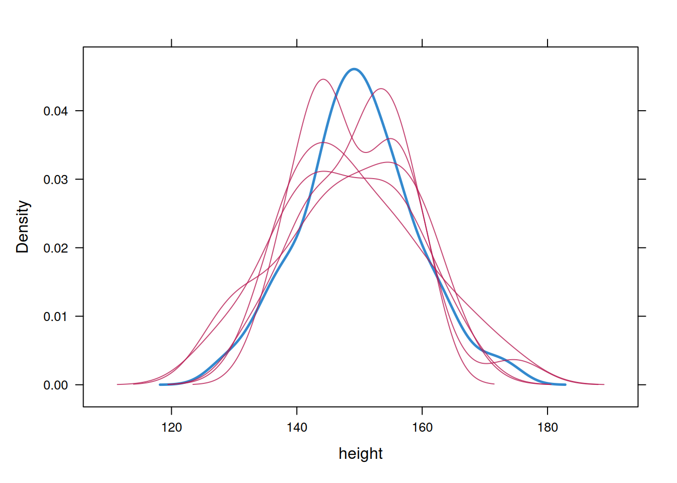
  packages = "miceadds")

9 Imputation Diagnostics

9.1 Logged Events

Code

mi_mice$loggedEvents

NULL

9.2 Trace Plots

On convergence, the streams of the trace plots should intermingle and be free of any trend (at the later iterations). Convergence is diagnosed when the variance between different sequences is no larger than the variance within each individual sequence.

https://stefvanbuuren.name/fimd/sec-algoptions.html (archived at https://perma.cc/4S54-465R)

Code

plot(mi_mice, c("height"))

9.3 Density Plots

Code

densityplot(mi_mice)

Code

densityplot(mi_mice, ~ height)

9.4 Strip Plots

Code

stripplot(mi_mice)

Code

stripplot(mi_mice, height ~ .imp)

10 Post-Processing

10.1 Modify/Create New Variables

10.1.1 `mice`

Code

mi_mice_long <- complete(
  mi_mice,
  action = "long",
  include = TRUE)

mi_mice_long$newVar <- mi_mice_long$age * mi_mice_long$height

10.1.2 `jomo`

Code

mi_jomo <- mi_jomo %>% 
  rename(height = dataToImpute...level1Vars.)

mi_jomo$newVar <- mi_jomo$age * mi_jomo$height

10.1.3 `Amelia`

Code

for(i in 1:length(mi_amelia$imputations)){
  mi_amelia$imputations[[i]]$newVar <- mi_amelia$imputations[[i]]$age * mi_amelia$imputations[[i]]$height
}

10.2 Convert to `mids` object

10.2.1 `mice`

Code

mi_mice_mids <- as.mids(mi_mice_long)

10.2.2 `jomo`

Code

mi_jomo_mids <- miceadds::jomo2mids(mi_jomo)

10.2.3 `Amelia`

Code

mi_amelia_mids <- miceadds::datlist2mids(mi_amelia$imputations)

10.3 Export for `Mplus`

Code

mids2mplus(mi_mice_mids, path = file.path("InsertFilePathHere", fsep = ""))
mids2mplus(mi_jomo_mids, path = file.path("InsertFilePathHere", fsep = ""))
mids2mplus(mi_amelia_mids, path = file.path("InsertFilePathHere", fsep = ""))

11 Fit Model to Multiply Imputed Data

11.1 Multiple Regression

Code

fit_lm <- with(
  data = mi_mice,
  expr = lm(height ~ age + Occasion))

11.1.1 Pool Results Across Models

Code

fit_lm_pooled <- mice::pool(fit_lm)

fit_lm_pooled

Error:
! arguments imply differing number of rows: 1, 0

Code

summary(fit_lm_pooled)

11.2 Mixed Model

Code

fit_lmer <- with(
  data = mi_mice,
  expr = lme4::lmer(height ~ age + Occasion + (1|id)))

11.2.1 Pool Results Across Models

Code

fit_lmer_pooled <- mice::pool(fit_lmer)

fit_lmer_pooled

Error:
! arguments imply differing number of rows: 1, 0

Code

summary(fit_lmer_pooled)

12 Model-Implied Predictions

Code

mice::predict_mi(
  fit_lm,
  #newdata = # can include if want to make predictions based on another (i.e., "new") data object
  se.fit = TRUE,
  interval = c("prediction")
)

$fit
       fit      lwr      upr
1 143.0912 126.6977 159.4847
2 144.7508 128.3986 161.1030
3 146.0963 129.7770 162.4156
4 147.3095 130.8591 163.7599
5 149.8360 133.5256 166.1463
6 151.5224 135.2058 167.8390

$se.fit
[1] 1.1025053 0.9291539 0.7638337 1.3045752 0.7125974 0.7486208

$df
[1]  1460.8931  1415.7428   637.8606   935.7190  6385.4620 20758.0027

$residual.scale
[1] 8.290191

Code

mice::predict_mi(
  fit_lmer,
  #newdata = # can include if want to make predictions based on another (i.e., "new") data object
  se.fit = TRUE,
  interval = c("prediction")
)

Error in `predict_mi.mira()`:
! `predict_mi()` currently only works with the linear model.

Error in `predict_mi.mira()`:
! `predict_mi()` currently only works with the linear model.

13 Resources

https://stefvanbuuren.name/fimd (archived at https://perma.cc/46U2-QTM6)

https://www.gerkovink.com/miceVignettes/Multi_level/Multi_level_data.html (archived at https://perma.cc/SF32-D7ZF)

14 Session Info

Code

sessionInfo()

R version 4.5.2 (2025-10-31)
Platform: x86_64-pc-linux-gnu
Running under: Ubuntu 24.04.3 LTS

Matrix products: default
BLAS:   /usr/lib/x86_64-linux-gnu/openblas-pthread/libblas.so.3 
LAPACK: /usr/lib/x86_64-linux-gnu/openblas-pthread/libopenblasp-r0.3.26.so;  LAPACK version 3.12.0

locale:
 [1] LC_CTYPE=C.UTF-8       LC_NUMERIC=C           LC_TIME=C.UTF-8       
 [4] LC_COLLATE=C.UTF-8     LC_MONETARY=C.UTF-8    LC_MESSAGES=C.UTF-8   
 [7] LC_PAPER=C.UTF-8       LC_NAME=C              LC_ADDRESS=C          
[10] LC_TELEPHONE=C         LC_MEASUREMENT=C.UTF-8 LC_IDENTIFICATION=C   

time zone: UTC
tzcode source: system (glibc)

attached base packages:
[1] stats     graphics  grDevices utils     datasets  methods   base     

other attached packages:
 [1] MplusAutomation_1.2 broom.mixed_0.2.9.6 lme4_1.1-38        
 [4] Matrix_1.7-4        nlme_3.1-168        furrr_0.3.1        
 [7] future_1.68.0       parallelly_1.46.0   jomo_2.7-6         
[10] Amelia_1.8.3        Rcpp_1.1.0          mitml_0.4-5        
[13] miceadds_3.18-36    micemd_1.10.1       mice_3.19.0        
[16] psych_2.5.6         lubridate_1.9.4     forcats_1.0.1      
[19] stringr_1.6.0       dplyr_1.1.4         purrr_1.2.0        
[22] readr_2.1.6         tidyr_1.3.2         tibble_3.3.0       
[25] ggplot2_4.0.1       tidyverse_2.0.0    

loaded via a namespace (and not attached):
  [1] RColorBrewer_1.1-3  jsonlite_2.0.0      GJRM_0.2-6.8       
  [4] shape_1.4.6.1       magrittr_2.0.4      farver_2.1.2       
  [7] nloptr_2.2.1        rmarkdown_2.30      vctrs_0.6.5        
 [10] minqa_1.2.8         htmltools_0.5.9     survey_4.4-8       
 [13] broom_1.0.11        htmlwidgets_1.6.4   gsubfn_0.7         
 [16] plyr_1.8.9          copula_1.1-6        sfsmisc_1.1-23     
 [19] lifecycle_1.0.4     startupmsg_1.0.0    iterators_1.0.14   
 [22] pkgconfig_2.0.3     R6_2.6.1            fastmap_1.2.0      
 [25] rbibutils_2.4       magic_1.6-1         digest_0.6.39      
 [28] numDeriv_2016.8-1.1 ismev_1.43          timechange_0.3.0   
 [31] pspline_1.0-21      httr_1.4.7          abind_1.4-8        
 [34] mgcv_1.9-3          compiler_4.5.2      mvmeta_1.0.3       
 [37] pander_0.6.6        withr_3.0.2         gsl_2.1-9          
 [40] S7_0.2.1            backports_1.5.0     DBI_1.2.3          
 [43] fastDummies_1.7.5   pan_1.9             MASS_7.3-65        
 [46] distr_2.9.7         VineCopula_2.6.1    tools_4.5.2        
 [49] pbivnorm_0.6.0      foreign_0.8-90      trust_0.1-8        
 [52] otel_0.2.0          nnet_7.3-20         glue_1.8.0         
 [55] stabledist_0.7-2    grid_4.5.2          checkmate_2.3.3    
 [58] generics_0.1.4      gtable_0.3.6        tzdb_0.5.0         
 [61] data.table_1.17.8   hms_1.1.4           foreach_1.5.2      
 [64] pillar_1.11.1       mitools_2.4         splines_4.5.2      
 [67] lattice_0.22-7      survival_3.8-3      gmp_0.7-5          
 [70] tidyselect_1.2.1    ADGofTest_0.3       knitr_1.51         
 [73] reformulas_0.4.3    stats4_4.5.2        xfun_0.55          
 [76] mixmeta_1.2.2       texreg_1.39.4       matrixStats_1.5.0  
 [79] proto_1.0.0         scam_1.2-20         stringi_1.8.7      
 [82] VGAM_1.1-14         yaml_2.3.12         boot_1.3-32        
 [85] evaluate_1.0.5      codetools_0.2-20    evd_2.3-7.1        
 [88] cli_3.6.5           rpart_4.1.24        xtable_1.8-4       
 [91] Rdpack_2.6.4        distrEx_2.9.6       globals_0.18.0     
 [94] coda_0.19-4.1       parallel_4.5.2      listenv_0.10.0     
 [97] gamlss.dist_6.1-1   Rmpfr_1.1-2         glmnet_4.1-10      
[100] mvtnorm_1.3-3       scales_1.4.0        pcaPP_2.0-5        
[103] rlang_1.1.6         mnormt_2.1.1

Reuse

CC BY 4.0

1 Preamble

1.1 Install Libraries

1.2 Load Libraries

1.3 Data

2 Types of Missingness

3 Approaches to Handle Missing Data

3.1 For MCAR/MAR Missingness

3.2 For MNAR Missingness

4 Approaches to Multiple Imputation

5 Describe Missing Data

6 Pre-Imputation Setup

6.1 Specify Variables to Impute

6.2 Specify Number of Imputations

6.3 Detect Cores

7 Multilevel Multiple Imputation

7.1 Three-Level and Cross-Classified Data

7.2 Methods

7.2.1 mice

7.2.1.1 Types

7.2.1.1.1 Continuous Outcomes

7.2.1.1.2 Binary Outcomes

7.2.1.1.3 Ordinal Outcomes

7.2.1.1.4 Count Outcomes

7.2.1.2 Specifying the Imputation Method

7.2.1.3 Specifying the Predictor Matrix

7.2.1.4 Syntax

7.2.2 jomo

7.2.3 Amelia

7.2.4 Mplus

7.2.4.1 Save Mplus Data File

7.2.4.2 Mplus Syntax for Multilevel Imputation

8 Parallel Processing

9 Imputation Diagnostics

9.1 Logged Events

9.2 Trace Plots

9.3 Density Plots

9.4 Strip Plots

10 Post-Processing

10.1 Modify/Create New Variables

10.1.1 mice

10.1.2 jomo

10.1.3 Amelia

10.2 Convert to mids object

10.2.1 mice

10.2.2 jomo

10.2.3 Amelia

10.3 Export for Mplus

11 Fit Model to Multiply Imputed Data

11.1 Multiple Regression

11.1.1 Pool Results Across Models

11.2 Mixed Model

11.2.1 Pool Results Across Models

12 Model-Implied Predictions

13 Resources

14 Session Info

Reuse

7.2.1 `mice`

7.2.2 `jomo`

7.2.3 `Amelia`

7.2.4 `Mplus`

7.2.4.1 Save `Mplus` Data File

7.2.4.2 `Mplus` Syntax for Multilevel Imputation

10.1.1 `mice`

10.1.2 `jomo`

10.1.3 `Amelia`

10.2 Convert to `mids` object

10.2.1 `mice`

10.2.2 `jomo`

10.2.3 `Amelia`

10.3 Export for `Mplus`