Data Management

1 Import Data

Importing data takes syntax of the following form for .csv files:

Code

data <- read.csv("filepath/filename.csv")

Note: it is important to use forward slashes (“/”) rather than backslashes (“\”) when specifying filepaths in R.

Below, I import a .csv file and save it into an object called mydata (you could call this object whatever you want):

Code

mydata <- read.csv("https://osf.io/s6wrm/download")

Importing data takes syntax of the following form for .RData files:

Code

load("filepath/filename.RData")

1.1 Import Multiple Data Files

Code

dataNames <- paste("data", 1:100, sep = "")
dataFilenames <- paste(dataNames, ".csv", sep = "")
dataFilepaths <- paste("C:/users/username/", dataFilenames, sep = "")

data_list <- lapply(dataFilepaths, read.csv) # lapply(dataFilepaths, data.table::fread) is even faster
names(data_list) <- basename(dataFilepaths)

Alternatively, if you want to load all .csv files in a directory, you can identify the filenames programmatically:

Code

dataFilenames <- list.files(
  path = "C:/users/username/",
  pattern = "\\.csv$")

dataFilepaths <- list.files(
  path = "C:/users/username/",
  pattern = "\\.csv$",
  full.names = TRUE)

data_list <- lapply(dataFilepaths, read.csv) # lapply(dataFilepaths, data.table::fread) is even faster
names(data_list) <- basename(dataFilepaths)

2 Save Data

Saving data takes syntax of the following form for .csv files:

Code

write.csv(object, file = "filepath/filename.csv")

For example:

Code

write.csv(mydata, file = "mydata.csv")

Saving data takes syntax of the following form for .RData files:

Code

save(object, file = "filepath/filename.RData")

3 Use Lab Functions

To use lab functions, first install the petersenlab package. The petersenlab package is here: https://devpsylab.github.io/petersenlab. You can install it using the following commands:

Code

install.packages("remotes")
remotes::install_github("DevPsyLab/petersenlab")

Once you have the petersenlab package installed, load the package:

Code

library("petersenlab")

To run scripts on the lab drive, set the path to the lab drive (//lc-rs-store24.hpc.uiowa.edu/lss_itpetersen/Lab/) using the following code:

Code

petersenLabPath <- setLabPath()

4 Load/Install Packages

To install a single package that is on the CRAN repository, use the following syntax:

Code

install.packages("name_of_package")

To install multiple packages that are on the CRAN repository, use the following syntax:

Code

install.packages(c("name_of_package1","name_of_package2","name_of_package3"))

To install a package that is on a GitHub repository, use the following syntax:

Code

install.packages("remotes")
remotes::install_github("username_of_GitHub_author/name_of_package")

For instance:

Code

remotes::install_github("DevPsyLab/petersenlab")

The default way to load a package in R is:

Code

library("packageName1")
library("packageName2")
library("packageName3")

However, when sourcing (i.e., running) other R scripts, it is possible that you will run scripts that use packages that you do not have installed, resulting in an error that prevents the script from running. Thus, it can be safer to load packages using the lab function, load_or_install(), rather than using library(). The load_or_install() function checks whether a package is installed. If the package is not installed, the function installs and loads the package. If the package is installed, the function loads the package. To use this function, you must have the petersenlab package loaded.

Code

library("petersenlab")
load_or_install(c("packageName1","packageName2","packageName3"))

For example:

Code

library("petersenlab")
load_or_install(c("tidyverse","psych"))

5 Set a Seed

Set a seed (any number) to reproduce the results of analyses that involve random number generation.

Code

set.seed(52242)

6 Run an `R` Script

To run an R script, use the following syntax:

Code

source("filepath/filename.R")

7 Render an `R` Markdown (`.Rmd`) File

To render a .Rmd file, use the following syntax:

Code

render("filepath/filename.Rmd")

8 Variable Names

To look at the names of variables in a data frame, use the following syntax:

Code

names(mydata)

[1] "survived"   "pclass"     "sex"        "age"        "sibsp"     
[6] "parch"      "prediction"

9 Logical Operators

Logical operators evaluate a condition for each value and yield values of TRUE and FALSE, corresponding to whether the evaluation for a given value met the condition.

9.1 Is Equal To: `==`

Code

mydata$survived == 1

[1]  TRUE  TRUE FALSE FALSE FALSE  TRUE

9.2 Is Not Equal To: `!=`

Code

mydata$survived != 1

[1] FALSE FALSE  TRUE  TRUE  TRUE FALSE

9.3 Greater Than: `>`

Code

mydata$parch > 1

[1] FALSE  TRUE  TRUE  TRUE  TRUE FALSE

9.4 Less Than: `<`

Code

mydata$parch < 1

[1]  TRUE FALSE FALSE FALSE FALSE  TRUE

9.5 Greater Than or Equal To: `>=`

Code

mydata$parch >= 1

[1] FALSE  TRUE  TRUE  TRUE  TRUE FALSE

9.6 Less Than or Equal To: `<=`

Code

mydata$parch <= 1

[1]  TRUE FALSE FALSE FALSE FALSE  TRUE

9.7 Is in a Value of Another Vector: `%in%`

Code

anotherVector <- c(0,1)
mydata$parch %in% anotherVector

[1]  TRUE FALSE FALSE FALSE FALSE  TRUE

9.8 Is Not in a Value of Another Vector: `%ni%`

Note: this function is part of the petersenlab package and is not available in base R.

Code

mydata$parch %ni% anotherVector

[1] FALSE  TRUE  TRUE  TRUE  TRUE FALSE

9.9 Is Missing: `is.na()`

Code

is.na(mydata$prediction)

[1] FALSE FALSE FALSE FALSE FALSE FALSE

9.10 Is Not Missing: `!is.na()`

Code

!is.na(mydata$prediction)

[1] TRUE TRUE TRUE TRUE TRUE TRUE

9.11 And: `&`

Code

!is.na(mydata$prediction) & mydata$parch >= 1

[1] FALSE  TRUE  TRUE  TRUE  TRUE FALSE

9.12 Or: `|`

Code

is.na(mydata$prediction) | mydata$parch >= 1

[1] FALSE  TRUE  TRUE  TRUE  TRUE FALSE

10 If…Else Conditions

We can use the construction, if()...else if()...else() if we want to perform conditional operations. The typical construction of if()...else if()...else() operates such that it first checks if the first if() condition is true. If the first if() condition is true, it performs the operation specified and terminates the process. If the first if() condition is not true, it checks the else if() conditions in order until one of them is true. For the first true else if() condition, it performs the operation specified and terminates the process. If none of the else if() conditions is true, it performs the operation specified under else() and then terminates the process. The construction, if()...else if()...else() can only be used on one value at a time.

Code

score <- 15

if(score <= 10){ # check this condition first
  rank <- 1
  print(rank)
} else if(score <= 20){ # if first condition was not met, check this condition next
  rank <- 2
  print(rank)
} else if(score <= 30){ # if first condition was not met, check this condition next
  rank <- 3
  print(rank)
} else{ # if all other conditions were not met, then do this
  print("Not Applicable!")
}

[1] 2

To apply conditional operations to a vector, we can use the ifelse() function.

Code

score <- c(1, 10, 20, 40, 100)

rank <- ifelse(
  score <= 10, # check this condition
  1, # assign this value if true
  2) # assign this value if false

rank

[1] 1 1 2 2 2

11 Subset

To subset a data frame, use brackets to specify the subset of rows and columns to keep, where the value/vector before the comma specifies the rows to keep, and the value/vector after the comma specifies the columns to keep:

Code

dataframe[rowsToKeep, columnsToKeep]

You can subset by using any of the following:

numeric indices of the rows/columns to keep (or drop)
names of the rows/columns to keep (or drop)
values of TRUE and FALSE corresponding to which rows/columns to keep

11.1 One Variable

To subset one variable, use the following syntax:

Code

mydata$age

[1] 29.00  0.92  2.00 30.00 25.00 48.00

or:

Code

mydata[,"age"]

[1] 29.00  0.92  2.00 30.00 25.00 48.00

11.2 Particular Rows of One Variable

To subset one variable, use the following syntax:

Code

mydata$age[which(mydata$survived == 1)]

[1] 29.00  0.92 48.00 63.00 53.00 18.00

or:

Code

mydata[which(mydata$survived == 1), "age"]

[1] 29.00  0.92 48.00 63.00 53.00 18.00

11.3 Particular Columns (Variables)

To subset particular columns/variables, use the following syntax:

11.3.1 Base `R`

Code

subsetVars <- c("survived","age","prediction")

mydata[,c(1,2,3)]

Code

mydata[,c("survived","age","prediction")]

Code

mydata[,subsetVars]

Or, to drop columns:

Code

dropVars <- c("sibsp","parch")

mydata[,-c(5,6)]

Code

mydata[,names(mydata) %ni% c("sibsp","parch")]

Code

mydata[,names(mydata) %ni% dropVars]

11.3.2 Tidyverse

Code

mydata %>%
  select(survived, age, prediction)

Code

mydata %>%
  select(survived:prediction)

Code

mydata %>%
  select(all_of(subsetVars))

Or, to drop columns:

Code

mydata %>%
  select(-sibsp, -parch)

Code

mydata %>%
  select(-c(sibsp:parch))

Code

mydata %>%
  select(-all_of(dropVars))

11.4 Particular Rows

To subset particular rows, use the following syntax:

11.4.1 Base `R`

Code

subsetRows <- c(1,3,5)

mydata[c(1,3,5),]

Code

mydata[subsetRows,]

Code

mydata[which(mydata$survived == 1),]

11.4.2 Tidyverse

Code

mydata %>%
  filter(survived == 1)

Code

mydata %>%
  filter(survived == 1, parch <= 1)

Code

mydata %>%
  filter(survived == 1 | parch <= 1)

11.5 Particular Rows and Columns

To subset particular rows and columns, use the following syntax:

11.5.1 Base `R`

Code

mydata[c(1,3,5), c(1,2,3)]

Code

mydata[subsetRows, subsetVars]

Code

mydata[which(mydata$survived == 1), subsetVars]

11.5.2 Tidyverse

Code

mydata %>%
  filter(survived == 1) %>%
  select(all_of(subsetVars))

12 View Data

12.1 All Data

To view data, use the following syntax:

Code

View(mydata)

12.2 First 6 Rows/Elements

To view only the first six rows (if a data frame) or elements (if a vector), use the following syntax:

Code

head(mydata)

Code

head(mydata$age)

[1] 29.00  0.92  2.00 30.00 25.00 48.00

13 Sort Data

Code

mydata %>% 
  arrange(survived, age) #sort by survived (ascending) then by age (ascending)

Code

mydata %>% 
  arrange(survived, -age) #sort by survived (ascending) then by age (descending)

14 Data Characteristics

14.1 Data Structure

Code

str(mydata)

'data.frame':   1046 obs. of  7 variables:
 $ survived  : int  1 1 0 0 0 1 1 0 1 0 ...
 $ pclass    : int  1 1 1 1 1 1 1 1 1 1 ...
 $ sex       : chr  "female" "male" "female" "male" ...
 $ age       : num  29 0.92 2 30 25 48 63 39 53 71 ...
 $ sibsp     : int  0 1 1 1 1 0 1 0 2 0 ...
 $ parch     : int  0 2 2 2 2 0 0 0 0 0 ...
 $ prediction: num  0.945 0.784 0.979 0.516 0.946 ...

14.2 Data Dimensions

Number of rows and columns:

Code

dim(mydata)

[1] 1046    7

14.3 Number of Elements

Code

length(mydata$age)

[1] 1046

14.4 Number of Missing Elements

Code

length(mydata$age[which(is.na(mydata$age))])

[1] 0

14.5 Number of Non-Missing Elements

Code

length(mydata$age[which(!is.na(mydata$age))])

[1] 1046

Code

length(na.omit(mydata$age))

[1] 1046

15 Create New Variables

To create a new variable, use the following syntax:

Code

mydata$newVar <- NA

Here is an example of creating a new variable:

Code

mydata$ID <- 1:nrow(mydata)

16 Create a Data Frame

Here is an example of creating a data frame:

Code

mydata2 <- data.frame(
  ID = c(1:5, 1047:1051),
  cat = sample(0:1, 10, replace = TRUE)
)

mydata2

17 Recode Variables

Here is an example of recoding a variable:

Code

mydata$oldVar1[which(mydata$sex == "male")] <- 0
mydata$oldVar1[which(mydata$sex == "female")] <- 1

mydata$oldVar2[which(mydata$sex == "male")] <- 1
mydata$oldVar2[which(mydata$sex == "female")] <- 0

Recode multiple variables:

Code

mydata %>%
  mutate(across(c(
    survived:pclass),
    ~ case_match(
      .,
      0 ~ "No",
      1 ~ "Yes")))

Code

mydata %>%
  mutate(across(c(
    survived:pclass),
    ~ case_match(
      .,
      c(0,1) ~ 1,
      c(2,3) ~ 2)))

18 Rename Variables

Code

mydata <- mydata %>% 
  rename(
    newVar1 = oldVar1,
    newVar2 = oldVar2)

Using a vector of variable names:

Code

varNamesFrom <- c("oldVar1","oldVar2")
varNamesTo <- c("newVar1","newVar2")

mydata <- mydata %>% 
  rename_with(~ varNamesTo, all_of(varNamesFrom))

19 Convert the Types of Variables

One variable:

Code

mydata$factorVar <- factor(mydata$sex)
mydata$numericVar <- as.numeric(mydata$prediction)
mydata$integerVar <- as.integer(mydata$parch)
mydata$characterVar <- as.character(mydata$sex)

Multiple variables:

Code

mydata %>%
  mutate(across(c(
    age,
    parch,
    prediction),
    as.numeric))

Code

mydata %>%
  mutate(across(
    age:parch,
    as.numeric))

Code

mydata %>%
  mutate(across(where(is.factor), as.character))

20 Merging/Joins

20.1 Overview

Merging (also called joining) merges two data objects using a shared set of variables called “keys.” The keys are the variable(s) that uniquely identify each row (i.e., they account for the levels of nesting). In some data objects, the key might be the participant’s ID (e.g., participantID). However, some data objects have multiple keys. For instance, in long form data objects, each participant may have multiple rows corresponding to multiple timepoints. In this case, the keys are participantID and timepoint. If a participant has multiple rows corresponding to timepoints and measures, the keys are participantID, timepoint, and measure. In general, each row should have a value on each of the keys; there should be no missingness in the keys.

To merge two objects, the keys must be present in both objects. The keys are used to merge the variables in object 1 (x) with the variables in object 2 (y). Different merge types select different rows to merge.

Note: if the two objects include variables with the same name (apart from the keys), R will not know how you want each to appear in the merged object. So, it will add a suffix (e.g., .x, .y) to each common variable to indicate which object (i.e., object x or object y) the variable came from, where object x is the first object—i.e., the object to which object y (the second object) is merged. In general, apart from the keys, you should not include variables with the same name in two objects to be merged. To prevent this, either remove or rename the shared variable in one of the objects, or include the shared variable as a key. However, as described above, you should include it as a key only if it uniquely identifies each row in terms of levels of nesting.

20.2 Data Before Merging

Here are the data in the mydata object:

Code

mydata

Code

dim(mydata)

[1] 1046   14

Here are the data in the mydata2 object:

Code

mydata2

Code

dim(mydata2)

[1] 10  2

20.3 Types of Joins

20.3.1 Visual Overview of Join Types

Below is a visual that depicts various types of merges/joins. Object x is the circle labeled as A. Object y is the circle labeled as B. The area of overlap in the Venn diagram indicates the rows on the keys that are shared between the two objects (e.g., participantID values 1, 2, and 3). The non-overlapping area indicates the rows on the keys that are unique to each object (e.g., participantID values 4, 5, and 6 in Object x and values 7, 8, and 9 in Object y). The shaded yellow area indicates which rows (on the keys) are kept in the merged object from each of the two objects, when using each of the merge types. For instance, a left outer join keeps the shared rows and the rows that are unique to object x, but it drops the rows that are unique to object y.

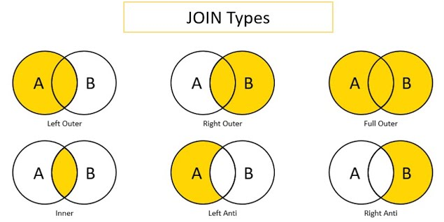
Image source: Predictive Hacks (archived at: https://perma.cc/WV7U-BS68)

20.3.2 Full Outer Join

A full outer join includes all rows in $x$ or $y$. It returns columns from $x$ and $y$. Here is how to merge two data frames using a full outer join (i.e., “full join”):

Code

fullJoinData <- merge(mydata, mydata2, by = "ID", all = TRUE)

fullJoinData

Code

dim(fullJoinData)

[1] 1051   15

Or, alternatively, using tidyverse:

Code

full_join(mydata, mydata2, by = "ID")

20.3.3 Left Outer Join

A left outer join includes all rows in $x$. It returns columns from $x$ and $y$. Here is how to merge two data frames using a left outer join (“left join”):

Code

leftJoinData <- merge(mydata, mydata2, by = "ID", all.x = TRUE)

leftJoinData

Code

dim(leftJoinData)

[1] 1046   15

Or, alternatively, using tidyverse:

Code

left_join(mydata, mydata2, by = "ID")

20.3.4 Right Outer Join

A right outer join includes all rows in $y$. It returns columns from $x$ and $y$. Here is how to merge two data frames using a right outer join (“right join”):

Code

rightJoinData <- merge(mydata, mydata2, by = "ID", all.y = TRUE)

rightJoinData

Code

dim(rightJoinData)

[1] 10 15

Or, alternatively, using tidyverse:

Code

right_join(mydata, mydata2, by = "ID")

20.3.5 Inner Join

An inner join includes all rows that are in both $x$ and $y$. An inner join will return one row of $x$ for each matching row of $y$, and can duplicate values of records on either side (left or right) if $x$ and $y$ have more than one matching record. It returns columns from $x$ and $y$. Here is how to merge two data frames using an inner join:

Code

innerJoinData <- merge(mydata, mydata2, by = "ID", all.x = FALSE, all.y = FALSE)

innerJoinData

Code

dim(innerJoinData)

[1]  5 15

Or, alternatively, using tidyverse:

Code

inner_join(mydata, mydata2, by = "ID")

20.3.6 Semi Join

A semi join is a filter. A left semi join returns all rows from $x$ with a match in $y$. That is, it filters out records from $x$ that are not in $y$. Unlike an inner join, a left semi join will never duplicate rows of $x$, and it includes columns from only $x$ (not from $y$). Here is how to merge two data frames using a left semi join:

Code

semiJoinData <- semi_join(mydata, mydata2, by = "ID")

semiJoinData

Code

dim(semiJoinData)

[1]  5 14

20.3.7 Anti Join

An anti join is a filter. A left anti join returns all rows from $x$ without a match in $y$. That is, it filters out records from $x$ that are in $y$. It returns columns from only $x$ (not from $y$). Here is how to merge two data frames using a left anti join:

Code

antiJoinData <- anti_join(mydata, mydata2, by = "ID")

antiJoinData

Code

dim(antiJoinData)

[1] 1041   14

20.3.8 Cross Join

A cross join combines each row in $x$ with each row in $y$.

Code

crossJoinData <- cross_join(
  data.frame(rater = c("Mother","Father","Teacher")),
  data.frame(timepoint = 1:3))

crossJoinData

Code

dim(crossJoinData)

[1] 9 2

21 Long to Wide

Original data:

Code

fish_encounters

Data widened by a variable (station), using tidyverse:

Code

fish_encounters %>% 
  pivot_wider(
    names_from = station,
    values_from = seen)

22 Wide to Long

Original data:

Code

mtcars

Data in long form, transformed from wide form using tidyverse:

Code

mtcars %>% 
  pivot_longer(
    cols = everything(),
    names_to = "variable",
    values_to = "value")

23 Average Ratings Across Coders

Create data with multiple coders:

Code

idWaveCoder <- 
  expand.grid(
    id = 1:100,
    wave = 1:3,
    coder = 1:3,
    positiveAffect = NA,
    negativeAffect = NA
  )

idWaveCoder$positiveAffect <- rnorm(nrow(idWaveCoder))
idWaveCoder$negativeAffect <- rnorm(nrow(idWaveCoder))

idWaveCoder %>% 
  arrange(id, wave, coder)

Average data across coders:

Code

idWave <- idWaveCoder %>% 
  group_by(id, wave) %>% 
  summarise(
    across(everything(),
      ~ mean(.x, na.rm = TRUE)),
    .groups = "drop") %>% 
  select(-coder)

idWave

24 Loops

If you want to perform the same computation multiple times, it can be faster to do it in a loop compared to writing out the same computation many times. For instance, here is a loop that prints each element of a vector and the loop index (i) that indicates where the loop is in terms of its iterations:

Code

fruits <- c("apple", "banana", "cherry")

for(i in 1:length(fruits)){
  print(paste("The loop is at index:", i, sep = " "))
  print(fruits[i])
}

[1] "The loop is at index: 1"
[1] "apple"
[1] "The loop is at index: 2"
[1] "banana"
[1] "The loop is at index: 3"
[1] "cherry"

24.1 Create a Function

Now, let’s put together what we have learned to create a useful function. Functions are useful if you want to perform an operation multiple times. Any operation that you want to perform multiple times, you can create a function to accomplish. Use of a function can save you time without needed to retype out all of the code each time. For instance, let’s say you want to convert temperature between Fahrenheit and Celsius, you could create a function to do that. In this case, our function has two arguments: temperature (in degrees) and unit of the original temperature (F for Fahrenheit or C for Celsius, where the default unit is Fahrenheit).

Code

convert_temperature <- function(temperature, unit = "F"){
  if(unit == "F"){ # if the input temperature(s) in Fahrenheit
    newtemp <- (temperature - 32) / (9/5)
  } else if(unit == "C"){ # if the input temperature(s) in Celsius
    newtemp <- (temperature * (9/5)) + 32
  }
  
  return(newtemp)
}

Now we can use the function to convert temperatures between Fahrenheit and Celsius. A temperature of 32°F is equal to 0°C. A temperature of 0°C is equal to 89.6°F.

Code

convert_temperature(
  temperature = 32,
  unit = "F"
)

[1] 0

Code

convert_temperature(
  temperature = 32,
  unit = "C"
)

[1] 89.6

We can also convert the temperature for a vector of values at once:

Code

convert_temperature(
  temperature = c(0, 10, 20, 30, 40, 50),
  unit = "F"
)

[1] -17.777778 -12.222222  -6.666667  -1.111111   4.444444  10.000000

Code

convert_temperature(
  temperature = c(0, 10, 20, 30, 40, 50),
  unit = "C"
)

[1]  32  50  68  86 104 122

Because the default unit is “F”, we do not need to specify the unit if our input temperatures are in Fahrenheit:

Code

convert_temperature(
  c(0, 10, 20, 30, 40, 50)
)

[1] -17.777778 -12.222222  -6.666667  -1.111111   4.444444  10.000000

25 Session Info

Code

sessionInfo()

R version 4.5.2 (2025-10-31)
Platform: x86_64-pc-linux-gnu
Running under: Ubuntu 24.04.3 LTS

Matrix products: default
BLAS:   /usr/lib/x86_64-linux-gnu/openblas-pthread/libblas.so.3 
LAPACK: /usr/lib/x86_64-linux-gnu/openblas-pthread/libopenblasp-r0.3.26.so;  LAPACK version 3.12.0

locale:
 [1] LC_CTYPE=C.UTF-8       LC_NUMERIC=C           LC_TIME=C.UTF-8       
 [4] LC_COLLATE=C.UTF-8     LC_MONETARY=C.UTF-8    LC_MESSAGES=C.UTF-8   
 [7] LC_PAPER=C.UTF-8       LC_NAME=C              LC_ADDRESS=C          
[10] LC_TELEPHONE=C         LC_MEASUREMENT=C.UTF-8 LC_IDENTIFICATION=C   

time zone: UTC
tzcode source: system (glibc)

attached base packages:
[1] stats     graphics  grDevices utils     datasets  methods   base     

other attached packages:
 [1] psych_2.5.6       lubridate_1.9.4   forcats_1.0.1     stringr_1.6.0    
 [5] dplyr_1.1.4       purrr_1.2.0       readr_2.1.6       tidyr_1.3.2      
 [9] tibble_3.3.0      ggplot2_4.0.1     tidyverse_2.0.0   petersenlab_1.2.2

loaded via a namespace (and not attached):
 [1] tidyselect_1.2.1   viridisLite_0.4.2  farver_2.1.2       S7_0.2.1          
 [5] fastmap_1.2.0      digest_0.6.39      rpart_4.1.24       timechange_0.3.0  
 [9] lifecycle_1.0.4    cluster_2.1.8.1    magrittr_2.0.4     compiler_4.5.2    
[13] rlang_1.1.6        Hmisc_5.2-4        tools_4.5.2        yaml_2.3.12       
[17] data.table_1.18.0  knitr_1.51         htmlwidgets_1.6.4  mnormt_2.1.1      
[21] plyr_1.8.9         RColorBrewer_1.1-3 foreign_0.8-90     withr_3.0.2       
[25] nnet_7.3-20        grid_4.5.2         stats4_4.5.2       lavaan_0.6-21     
[29] xtable_1.8-4       colorspace_2.1-2   scales_1.4.0       MASS_7.3-65       
[33] cli_3.6.5          mvtnorm_1.3-3      rmarkdown_2.30     reformulas_0.4.3  
[37] generics_0.1.4     otel_0.2.0         rstudioapi_0.17.1  reshape2_1.4.5    
[41] tzdb_0.5.0         minqa_1.2.8        DBI_1.2.3          splines_4.5.2     
[45] parallel_4.5.2     base64enc_0.1-3    mitools_2.4        vctrs_0.6.5       
[49] boot_1.3-32        Matrix_1.7-4       jsonlite_2.0.0     hms_1.1.4         
[53] Formula_1.2-5      htmlTable_2.4.3    glue_1.8.0         nloptr_2.2.1      
[57] stringi_1.8.7      gtable_0.3.6       quadprog_1.5-8     lme4_1.1-38       
[61] pillar_1.11.1      htmltools_0.5.9    R6_2.6.1           Rdpack_2.6.4      
[65] mix_1.0-13         evaluate_1.0.5     pbivnorm_0.6.0     lattice_0.22-7    
[69] rbibutils_2.4      backports_1.5.0    Rcpp_1.1.0         gridExtra_2.3     
[73] nlme_3.1-168       checkmate_2.3.3    xfun_0.55          pkgconfig_2.0.3

Reuse

CC BY 4.0

--- title: "Data Management" output: html_document: code_folding: show --- # Import Data {#importData} Importing data takes syntax of the following form for `.csv` files: ```{r} #| eval: false data <- read.csv("filepath/filename.csv") ``` Note: it is important to use forward slashes ("/") rather than backslashes ("\\") when specifying filepaths in `R`. Below, I import a `.csv` file and save it into an object called `mydata` (you could call this object whatever you want): ```{r} #| eval: false mydata <- read.csv("https://osf.io/s6wrm/download") ``` ```{r} #| include: false mydata <- read.csv("./data/titanic.csv") #https://osf.io/s6wrm/download ``` Importing data takes syntax of the following form for `.RData` files: ```{r} #| eval: false load("filepath/filename.RData") ``` ## Import Multiple Data Files {#importMultipleDataFiles} ```{r} #| eval: false dataNames <- paste("data", 1:100, sep = "") dataFilenames <- paste(dataNames, ".csv", sep = "") dataFilepaths <- paste("C:/users/username/", dataFilenames, sep = "") data_list <- lapply(dataFilepaths, read.csv) # lapply(dataFilepaths, data.table::fread) is even faster names(data_list) <- basename(dataFilepaths) ``` Alternatively, if you want to load all `.csv` files in a directory, you can identify the filenames programmatically: ```{r} #| eval: false dataFilenames <- list.files( path = "C:/users/username/", pattern = "\\.csv$") dataFilepaths <- list.files( path = "C:/users/username/", pattern = "\\.csv$", full.names = TRUE) data_list <- lapply(dataFilepaths, read.csv) # lapply(dataFilepaths, data.table::fread) is even faster names(data_list) <- basename(dataFilepaths) ``` # Save Data {#saveData} Saving data takes syntax of the following form for `.csv` files: ```{r} #| eval: false write.csv(object, file = "filepath/filename.csv") ``` For example: ```{r} #| eval: false write.csv(mydata, file = "mydata.csv") ``` Saving data takes syntax of the following form for `.RData` files: ```{r} #| eval: false save(object, file = "filepath/filename.RData") ``` # Use Lab Functions {#labFunctions} To use lab functions, first install the [`petersenlab` package](https://devpsylab.github.io/petersenlab). The [`petersenlab` package](https://devpsylab.github.io/petersenlab) is here: <https://devpsylab.github.io/petersenlab>. You can install it using the following commands: ```{r} #| eval: false install.packages("remotes") remotes::install_github("DevPsyLab/petersenlab") ``` Once you have the [`petersenlab` package](https://devpsylab.github.io/petersenlab) installed, load the package: ```{r} library("petersenlab") ``` To run scripts on the lab drive, set the path to the lab drive (`//lc-rs-store24.hpc.uiowa.edu/lss_itpetersen/Lab/`) using the following code: ```{r} #| eval: false petersenLabPath <- setLabPath() ``` # Load/Install Packages {#loadInstallPackages} To install a single package that is on the CRAN repository, use the following syntax: ```{r} #| eval: false install.packages("name_of_package") ``` To install multiple packages that are on the CRAN repository, use the following syntax: ```{r} #| eval: false install.packages(c("name_of_package1","name_of_package2","name_of_package3")) ``` To install a package that is on a `GitHub` repository, use the following syntax: ```{r} #| eval: false install.packages("remotes") remotes::install_github("username_of_GitHub_author/name_of_package") ``` For instance: ```{r} #| eval: false remotes::install_github("DevPsyLab/petersenlab") ``` The default way to load a package in `R` is: ```{r} #| eval: false library("packageName1") library("packageName2") library("packageName3") ``` However, when sourcing (i.e., running) other `R` scripts, it is possible that you will run scripts that use packages that you do not have installed, resulting in an error that prevents the script from running. Thus, it can be safer to load packages using the lab function, `load_or_install(),` rather than using `library()`. The `load_or_install()` function checks whether a package is installed. If the package is not installed, the function installs and loads the package. If the package is installed, the function loads the package. To use this function, you must have the [`petersenlab` package](https://devpsylab.github.io/petersenlab) loaded. ```{r} #| eval: false library("petersenlab") load_or_install(c("packageName1","packageName2","packageName3")) ``` For example: ```{r} library("petersenlab") load_or_install(c("tidyverse","psych")) ``` # Set a Seed {#seed} Set a seed (any number) to reproduce the results of analyses that involve random number generation. ```{r} set.seed(52242) ``` # Run an `R` Script {#source} To run an `R` script, use the following syntax: ```{r} #| eval: false source("filepath/filename.R") ``` # Render an `R` Markdown (`.Rmd`) File {#renderRmd} To render a `.Rmd` file, use the following syntax: ```{r} #| eval: false render("filepath/filename.Rmd") ``` # Variable Names {#varNames} To look at the names of variables in a data frame, use the following syntax: ```{r} names(mydata) ``` # Logical Operators {#logicalOperators} Logical operators evaluate a condition for each value and yield values of `TRUE` and `FALSE`, corresponding to whether the evaluation for a given value met the condition. ## Is Equal To: `==` ```{r} #| output: false mydata$survived == 1 ``` ```{r} #| echo: false head(mydata$survived == 1) ``` ## Is Not Equal To: `!=` ```{r} #| output: false mydata$survived != 1 ``` ```{r} #| echo: false head(mydata$survived != 1) ``` ## Greater Than: `>` ```{r} #| output: false mydata$parch > 1 ``` ```{r} #| echo: false head(mydata$parch > 1) ``` ## Less Than: `<` ```{r} #| output: false mydata$parch < 1 ``` ```{r} #| echo: false head(mydata$parch < 1) ``` ## Greater Than or Equal To: `>=` ```{r} #| output: false mydata$parch >= 1 ``` ```{r} #| echo: false head(mydata$parch >= 1) ``` ## Less Than or Equal To: `<=` ```{r} #| output: false mydata$parch <= 1 ``` ```{r} #| echo: false head(mydata$parch <= 1) ``` ## Is in a Value of Another Vector: `%in%` ```{r} #| output: false anotherVector <- c(0,1) mydata$parch %in% anotherVector ``` ```{r} #| echo: false head(mydata$parch %in% anotherVector) ``` ## Is Not in a Value of Another Vector: `%ni%` Note: this function is part of the [`petersenlab`](https://github.com/DevPsyLab/petersenlab) package and is not available in base `R`. ```{r} #| output: false mydata$parch %ni% anotherVector ``` ```{r} #| echo: false head(mydata$parch %ni% anotherVector) ``` ## Is Missing: `is.na()` ```{r} #| output: false is.na(mydata$prediction) ``` ```{r} #| echo: false head(is.na(mydata$prediction)) ``` ## Is Not Missing: `!is.na()` ```{r} #| output: false !is.na(mydata$prediction) ``` ```{r} #| echo: false head(!is.na(mydata$prediction)) ``` ## And: `&` ```{r} #| output: false !is.na(mydata$prediction) & mydata$parch >= 1 ``` ```{r} #| echo: false head(!is.na(mydata$prediction) & mydata$parch >= 1) ``` ## Or: `|` ```{r} #| output: false is.na(mydata$prediction) | mydata$parch >= 1 ``` ```{r} #| echo: false head(is.na(mydata$prediction) | mydata$parch >= 1) ``` # If...Else Conditions {#ifelse} We can use the construction, `if()...else if()...else()` if we want to perform conditional operations. The typical construction of `if()...else if()...else()` operates such that it first checks if the first `if()` condition is true. If the first `if()` condition is true, it performs the operation specified and terminates the process. If the first `if()` condition is not true, it checks the `else if()` conditions in order until one of them is true. For the first true `else if()` condition, it performs the operation specified and terminates the process. If none of the `else if()` conditions is true, it performs the operation specified under `else()` and then terminates the process. The construction, `if()...else if()...else()` can only be used on one value at a time. ```{r} score <- 15 if(score <= 10){ # check this condition first rank <- 1 print(rank) } else if(score <= 20){ # if first condition was not met, check this condition next rank <- 2 print(rank) } else if(score <= 30){ # if first condition was not met, check this condition next rank <- 3 print(rank) } else{ # if all other conditions were not met, then do this print("Not Applicable!") } ``` To apply conditional operations to a vector, we can use the `ifelse()` function. ```{r} score <- c(1, 10, 20, 40, 100) rank <- ifelse( score <= 10, # check this condition 1, # assign this value if true 2) # assign this value if false rank ``` # Subset {#subset} To subset a data frame, use brackets to specify the subset of rows and columns to keep, where the value/vector before the comma specifies the rows to keep, and the value/vector after the comma specifies the columns to keep: ```{r} #| eval: false dataframe[rowsToKeep, columnsToKeep] ``` You can subset by using any of the following: - numeric indices of the rows/columns to keep (or drop) - names of the rows/columns to keep (or drop) - values of `TRUE` and `FALSE` corresponding to which rows/columns to keep ## One Variable To subset one variable, use the following syntax: ```{r} #| output: false mydata$age ``` ```{r} #| echo: false head(mydata$age) ``` or: ```{r} #| output: false mydata[,"age"] ``` ```{r} #| echo: false head(mydata[,"age"]) ``` ## Particular Rows of One Variable To subset one variable, use the following syntax: ```{r} #| output: false mydata$age[which(mydata$survived == 1)] ``` ```{r} #| echo: false head(mydata$age[which(mydata$survived == 1)]) ``` or: ```{r} #| output: false mydata[which(mydata$survived == 1), "age"] ``` ```{r} #| echo: false head(mydata[which(mydata$survived == 1), "age"]) ``` ## Particular Columns (Variables) To subset particular columns/variables, use the following syntax: ### Base `R` ```{r} subsetVars <- c("survived","age","prediction") mydata[,c(1,2,3)] mydata[,c("survived","age","prediction")] mydata[,subsetVars] ``` Or, to drop columns: ```{r} dropVars <- c("sibsp","parch") mydata[,-c(5,6)] mydata[,names(mydata) %ni% c("sibsp","parch")] mydata[,names(mydata) %ni% dropVars] ``` ### Tidyverse ```{r} mydata %>% select(survived, age, prediction) mydata %>% select(survived:prediction) mydata %>% select(all_of(subsetVars)) ``` Or, to drop columns: ```{r} mydata %>% select(-sibsp, -parch) mydata %>% select(-c(sibsp:parch)) mydata %>% select(-all_of(dropVars)) ``` ## Particular Rows To subset particular rows, use the following syntax: ### Base `R` ```{r} subsetRows <- c(1,3,5) mydata[c(1,3,5),] mydata[subsetRows,] mydata[which(mydata$survived == 1),] ``` ### Tidyverse ```{r} mydata %>% filter(survived == 1) mydata %>% filter(survived == 1, parch <= 1) mydata %>% filter(survived == 1 | parch <= 1) ``` ## Particular Rows and Columns To subset particular rows and columns, use the following syntax: ### Base `R` ```{r} mydata[c(1,3,5), c(1,2,3)] mydata[subsetRows, subsetVars] mydata[which(mydata$survived == 1), subsetVars] ``` ### Tidyverse ```{r} mydata %>% filter(survived == 1) %>% select(all_of(subsetVars)) ``` # View Data {#viewData} ## All Data To view data, use the following syntax: ```{r} #| eval: false View(mydata) ``` ## First 6 Rows/Elements To view only the first six rows (if a data frame) or elements (if a vector), use the following syntax: ```{r} head(mydata) head(mydata$age) ``` # Sort Data {#sec-sortData} ```{r} mydata %>% arrange(survived, age) #sort by survived (ascending) then by age (ascending) mydata %>% arrange(survived, -age) #sort by survived (ascending) then by age (descending) ``` # Data Characteristics {#dataCharacteristics} ## Data Structure ```{r} str(mydata) ``` ## Data Dimensions Number of rows and columns: ```{r} dim(mydata) ``` ## Number of Elements ```{r} length(mydata$age) ``` ## Number of Missing Elements ```{r} length(mydata$age[which(is.na(mydata$age))]) ``` ## Number of Non-Missing Elements ```{r} length(mydata$age[which(!is.na(mydata$age))]) length(na.omit(mydata$age)) ``` # Create New Variables {#createNewVars} To create a new variable, use the following syntax: ```{r} mydata$newVar <- NA ``` ```{r} #| include: false mydata$newVar <- NULL ``` Here is an example of creating a new variable: ```{r} mydata$ID <- 1:nrow(mydata) ``` # Create a Data Frame {#createDF} Here is an example of creating a data frame: ```{r} mydata2 <- data.frame( ID = c(1:5, 1047:1051), cat = sample(0:1, 10, replace = TRUE) ) mydata2 ``` # Recode Variables {#recodeVars} Here is an example of recoding a variable: ```{r} mydata$oldVar1[which(mydata$sex == "male")] <- 0 mydata$oldVar1[which(mydata$sex == "female")] <- 1 mydata$oldVar2[which(mydata$sex == "male")] <- 1 mydata$oldVar2[which(mydata$sex == "female")] <- 0 ``` Recode multiple variables: ```{r} mydata %>% mutate(across(c( survived:pclass), ~ case_match( ., 0 ~ "No", 1 ~ "Yes"))) mydata %>% mutate(across(c( survived:pclass), ~ case_match( ., c(0,1) ~ 1, c(2,3) ~ 2))) ``` # Rename Variables {#renameVars} ```{r} mydata <- mydata %>% rename( newVar1 = oldVar1, newVar2 = oldVar2) ``` Using a vector of variable names: ```{r} #| eval: false varNamesFrom <- c("oldVar1","oldVar2") varNamesTo <- c("newVar1","newVar2") mydata <- mydata %>% rename_with(~ varNamesTo, all_of(varNamesFrom)) ``` # Convert the Types of Variables {#convertVarTypes} One variable: ```{r} mydata$factorVar <- factor(mydata$sex) mydata$numericVar <- as.numeric(mydata$prediction) mydata$integerVar <- as.integer(mydata$parch) mydata$characterVar <- as.character(mydata$sex) ``` Multiple variables: ```{r} mydata %>% mutate(across(c( age, parch, prediction), as.numeric)) mydata %>% mutate(across( age:parch, as.numeric)) mydata %>% mutate(across(where(is.factor), as.character)) ``` # Merging/Joins {#merging} ## Overview Merging (also called joining) merges two data objects using a shared set of variables called "keys." The keys are the variable(s) that uniquely identify each row (i.e., they account for the levels of nesting). In some data objects, the key might be the participant's ID (e.g., `participantID`). However, some data objects have multiple keys. For instance, in long form data objects, each participant may have multiple rows corresponding to multiple timepoints. In this case, the keys are `participantID` and `timepoint`. If a participant has multiple rows corresponding to timepoints and measures, the keys are `participantID`, `timepoint`, and `measure`. In general, each row should have a value on each of the keys; there should be no missingness in the keys. To merge two objects, the keys must be present in both objects. The keys are used to merge the variables in object 1 (`x`) with the variables in object 2 (`y`). Different merge types select different rows to merge. Note: if the two objects include variables with the same name (apart from the keys), `R` will not know how you want each to appear in the merged object. So, it will add a suffix (e.g., `.x`, `.y`) to each common variable to indicate which object (i.e., object `x` or object `y`) the variable came from, where object `x` is the first object—i.e., the object to which object `y` (the second object) is merged. In general, apart from the keys, you should not include variables with the same name in two objects to be merged. To prevent this, either remove or rename the shared variable in one of the objects, or include the shared variable as a key. However, as described above, you should include it as a key ***only*** if it uniquely identifies each row in terms of levels of nesting. ## Data Before Merging Here are the data in the `mydata` object: ```{r} mydata dim(mydata) ``` Here are the data in the `mydata2` object: ```{r} mydata2 dim(mydata2) ``` ## Types of Joins {#mergeTypes} ### Visual Overview of Join Types Below is a visual that depicts various types of merges/joins. Object `x` is the circle labeled as `A`. Object `y` is the circle labeled as `B`. The area of overlap in the Venn diagram indicates the rows on the keys that are shared between the two objects (e.g., `participantID` values 1, 2, and 3). The non-overlapping area indicates the rows on the keys that are unique to each object (e.g., `participantID` values 4, 5, and 6 in Object `x` and values 7, 8, and 9 in Object `y`). The shaded yellow area indicates which rows (on the keys) are kept in the merged object from each of the two objects, when using each of the merge types. For instance, a left outer join keeps the shared rows and the rows that are unique to object `x`, but it drops the rows that are unique to object `y`. ![Types of merges/joins](images/joins.png) Image source: [Predictive Hacks](https://predictivehacks.com/?all-tips=anti-joins-with-pandas) (archived at: <https://perma.cc/WV7U-BS68>) ### Full Outer Join {#fullJoin} A full outer join includes all rows in $x$ **or** $y$. It returns columns from $x$ and $y$. Here is how to merge two data frames using a full outer join (i.e., "full join"): ```{r} fullJoinData <- merge(mydata, mydata2, by = "ID", all = TRUE) fullJoinData dim(fullJoinData) ``` Or, alternatively, using `tidyverse`: ```{r} full_join(mydata, mydata2, by = "ID") ``` ### Left Outer Join {#leftJoin} A left outer join includes all rows in $x$. It returns columns from $x$ and $y$. Here is how to merge two data frames using a left outer join ("left join"): ```{r} leftJoinData <- merge(mydata, mydata2, by = "ID", all.x = TRUE) leftJoinData dim(leftJoinData) ``` Or, alternatively, using `tidyverse`: ```{r} left_join(mydata, mydata2, by = "ID") ``` ### Right Outer Join {#rightJoin} A right outer join includes all rows in $y$. It returns columns from $x$ and $y$. Here is how to merge two data frames using a right outer join ("right join"): ```{r} rightJoinData <- merge(mydata, mydata2, by = "ID", all.y = TRUE) rightJoinData dim(rightJoinData) ``` Or, alternatively, using `tidyverse`: ```{r} right_join(mydata, mydata2, by = "ID") ``` ### Inner Join {#innerJoin} An inner join includes all rows that are in **both** $x$ **and** $y$. An inner join will return one row of $x$ for each matching row of $y$, and can duplicate values of records on either side (left or right) if $x$ and $y$ have more than one matching record. It returns columns from $x$ and $y$. Here is how to merge two data frames using an inner join: ```{r} innerJoinData <- merge(mydata, mydata2, by = "ID", all.x = FALSE, all.y = FALSE) innerJoinData dim(innerJoinData) ``` Or, alternatively, using `tidyverse`: ```{r} inner_join(mydata, mydata2, by = "ID") ``` ### Semi Join {#semiJoin} A semi join is a filter. A left semi join returns all rows from $x$ **with** a match in $y$. That is, it filters out records from $x$ that are not in $y$. Unlike an [inner join](#innerJoin), a left semi join will never duplicate rows of $x$, and it includes columns from only $x$ (not from $y$). Here is how to merge two data frames using a left semi join: ```{r} semiJoinData <- semi_join(mydata, mydata2, by = "ID") semiJoinData dim(semiJoinData) ``` ### Anti Join {#antiJoin} An anti join is a filter. A left anti join returns all rows from $x$ **without** a match in $y$. That is, it filters out records from $x$ that are in $y$. It returns columns from only $x$ (not from $y$). Here is how to merge two data frames using a left anti join: ```{r} antiJoinData <- anti_join(mydata, mydata2, by = "ID") antiJoinData dim(antiJoinData) ``` ### Cross Join {#crossJoin} A cross join combines each row in $x$ with each row in $y$. ```{r} crossJoinData <- cross_join( data.frame(rater = c("Mother","Father","Teacher")), data.frame(timepoint = 1:3)) crossJoinData dim(crossJoinData) ``` # Long to Wide {#longToWide} Original data: ```{r} fish_encounters ``` Data widened by a variable (`station`), using `tidyverse`: ```{r} fish_encounters %>% pivot_wider( names_from = station, values_from = seen) ``` # Wide to Long {#wideToLong} Original data: ```{r} mtcars ``` Data in long form, transformed from wide form using `tidyverse`: ```{r} mtcars %>% pivot_longer( cols = everything(), names_to = "variable", values_to = "value") ``` # Average Ratings Across Coders {#avgAcrossCoders} Create data with multiple coders: ```{r} #| code-fold: true idWaveCoder <- expand.grid( id = 1:100, wave = 1:3, coder = 1:3, positiveAffect = NA, negativeAffect = NA ) idWaveCoder$positiveAffect <- rnorm(nrow(idWaveCoder)) idWaveCoder$negativeAffect <- rnorm(nrow(idWaveCoder)) idWaveCoder %>% arrange(id, wave, coder) ``` Average data across coders: ```{r} idWave <- idWaveCoder %>% group_by(id, wave) %>% summarise( across(everything(), ~ mean(.x, na.rm = TRUE)), .groups = "drop") %>% select(-coder) idWave ``` # Loops {#loops} If you want to perform the same computation multiple times, it can be faster to do it in a loop compared to writing out the same computation many times. For instance, here is a loop that prints each element of a vector and the loop index (`i`) that indicates where the loop is in terms of its iterations: ```{r} fruits <- c("apple", "banana", "cherry") for(i in 1:length(fruits)){ print(paste("The loop is at index:", i, sep = " ")) print(fruits[i]) } ``` ## Create a Function {#createFunction} Now, let's put together what we have learned to create a useful function. Functions are useful if you want to perform an operation multiple times. Any operation that you want to perform multiple times, you can create a function to accomplish. Use of a function can save you time without needed to retype out all of the code each time. For instance, let's say you want to convert temperature between Fahrenheit and Celsius, you could create a function to do that. In this case, our function has two arguments: `temperature` (in degrees) and `unit` of the original temperature (`F` for Fahrenheit or `C` for Celsius, where the default unit is Fahrenheit). ```{r} convert_temperature <- function(temperature, unit = "F"){ if(unit == "F"){ # if the input temperature(s) in Fahrenheit newtemp <- (temperature - 32) / (9/5) } else if(unit == "C"){ # if the input temperature(s) in Celsius newtemp <- (temperature * (9/5)) + 32 } return(newtemp) } ``` Now we can use the function to convert temperatures between Fahrenheit and Celsius. A temperature of 32°F is equal to 0°C. A temperature of 0°C is equal to 89.6°F. ```{r} convert_temperature( temperature = 32, unit = "F" ) convert_temperature( temperature = 32, unit = "C" ) ``` We can also convert the temperature for a vector of values at once: ```{r} convert_temperature( temperature = c(0, 10, 20, 30, 40, 50), unit = "F" ) convert_temperature( temperature = c(0, 10, 20, 30, 40, 50), unit = "C" ) ``` Because the default unit is "F", we do not need to specify the unit if our input temperatures are in Fahrenheit: ```{r} convert_temperature( c(0, 10, 20, 30, 40, 50) ) ``` # Session Info ```{r} #| code-fold: true sessionInfo() ```

1 Import Data

1.1 Import Multiple Data Files

2 Save Data

3 Use Lab Functions

4 Load/Install Packages

5 Set a Seed

6 Run an R Script

7 Render an R Markdown (.Rmd) File

8 Variable Names

9 Logical Operators

9.1 Is Equal To: ==

9.2 Is Not Equal To: !=

9.3 Greater Than: >

9.4 Less Than: <

9.5 Greater Than or Equal To: >=

9.6 Less Than or Equal To: <=

9.7 Is in a Value of Another Vector: %in%

9.8 Is Not in a Value of Another Vector: %ni%

9.9 Is Missing: is.na()

9.10 Is Not Missing: !is.na()

9.11 And: &

9.12 Or: |

10 If…Else Conditions

11 Subset

11.1 One Variable

11.2 Particular Rows of One Variable

11.3 Particular Columns (Variables)

11.3.1 Base R

11.3.2 Tidyverse

11.4 Particular Rows

11.4.1 Base R

11.4.2 Tidyverse

11.5 Particular Rows and Columns

11.5.1 Base R

11.5.2 Tidyverse

12 View Data

12.1 All Data

12.2 First 6 Rows/Elements

13 Sort Data

14 Data Characteristics

14.1 Data Structure

14.2 Data Dimensions

14.3 Number of Elements

14.4 Number of Missing Elements

14.5 Number of Non-Missing Elements

15 Create New Variables

16 Create a Data Frame

17 Recode Variables

18 Rename Variables

19 Convert the Types of Variables

20 Merging/Joins

20.1 Overview

20.2 Data Before Merging

20.3 Types of Joins

20.3.1 Visual Overview of Join Types

20.3.2 Full Outer Join

20.3.3 Left Outer Join

20.3.4 Right Outer Join

20.3.5 Inner Join

20.3.6 Semi Join

20.3.7 Anti Join

20.3.8 Cross Join

21 Long to Wide

22 Wide to Long

23 Average Ratings Across Coders

24 Loops

24.1 Create a Function

25 Session Info

Reuse

6 Run an `R` Script

7 Render an `R` Markdown (`.Rmd`) File

9.1 Is Equal To: `==`

9.2 Is Not Equal To: `!=`

9.3 Greater Than: `>`

9.4 Less Than: `<`

9.5 Greater Than or Equal To: `>=`

9.6 Less Than or Equal To: `<=`

9.7 Is in a Value of Another Vector: `%in%`

9.8 Is Not in a Value of Another Vector: `%ni%`

9.9 Is Missing: `is.na()`

9.10 Is Not Missing: `!is.na()`

9.11 And: `&`

9.12 Or: `|`

11.3.1 Base `R`

11.4.1 Base `R`

11.5.1 Base `R`