Code
#install.packages("remotes")
#remotes::install_github("DevPsyLab/petersenlab")#install.packages("remotes")
#remotes::install_github("DevPsyLab/petersenlab")library("petersenlab")
library("MASS")
library("tidyverse")
library("psych")
library("rms")
library("robustbase")
library("brms")
library("cvTools")
library("car")
library("mgcv")
library("AER")
library("foreign")
library("olsrr")
library("quantreg")
library("mblm")
library("effects")
library("correlation")
library("interactions")
library("lavaan")
library("regtools")
library("mice")
library("XICOR")
library("cocor")
library("effectsize")
library("rockchalk")
library("yhat")mydata <- read.csv("https://osf.io/8syp5/download")mydata$countVariable <- as.integer(mydata$bpi_antisocialT2Sum)
mydata$orderedVariable <- factor(mydata$countVariable, ordered = TRUE)
mydata$female <- NA
mydata$female[which(mydata$sex == "male")] <- 0
mydata$female[which(mydata$sex == "female")] <- 1https://isaactpetersen.github.io/Fantasy-Football-Analytics-Textbook/multiple-regression.html
Call:
lm(formula = bpi_antisocialT2Sum ~ bpi_antisocialT1Sum + bpi_anxiousDepressedSum,
    data = mydata, na.action = na.exclude)

Residuals:
    Min      1Q  Median      3Q     Max
-8.3755 -1.2337 -0.2212  0.9911 12.8017

Coefficients:
                        Estimate Std. Error t value Pr(>|t|)
(Intercept)              1.19830    0.05983  20.029  < 2e-16 ***
bpi_antisocialT1Sum      0.46553    0.01858  25.049  < 2e-16 ***
bpi_anxiousDepressedSum  0.16075    0.02916   5.513 3.83e-08 ***
---
Signif. codes:  0 '***' 0.001 '**' 0.01 '*' 0.05 '.' 0.1 ' ' 1

Residual standard error: 1.979 on 2871 degrees of freedom
  (8656 observations deleted due to missingness)
Multiple R-squared:  0.262, Adjusted R-squared:  0.2615
F-statistic: 509.6 on 2 and 2871 DF, p-value: < 2.2e-16confint(multipleRegressionModel) 2.5 % 97.5 %
(Intercept) 1.0809881 1.3156128
bpi_antisocialT1Sum 0.4290884 0.5019688
bpi_anxiousDepressedSum 0.1035825 0.2179258print(effectsize::standardize_parameters(multipleRegressionModel), digits = 2)# Standardization method: refit
Parameter | Std. Coef. | 95% CI
----------------------------------------------------
(Intercept) | 1.62e-16 | [-0.03, 0.03]
bpi antisocialT1Sum | 0.46 | [ 0.42, 0.49]
bpi anxiousDepressedSum | 0.10 | [ 0.06, 0.14]multipleRegressionModelNoMissing <- lm(
bpi_antisocialT2Sum ~ bpi_antisocialT1Sum + bpi_anxiousDepressedSum,
data = mydata,
na.action = na.omit)
multipleRegressionModelNoMissing <- lm(
bpi_antisocialT2Sum ~ bpi_antisocialT1Sum + bpi_anxiousDepressedSum,
data = mydata |> select(bpi_antisocialT2Sum, bpi_antisocialT1Sum, bpi_anxiousDepressedSum) |> na.omit)Error in na.omit: The pipe operator requires a function call as RHS (<input>:8:97)
summary(multipleRegressionModelPairwise)
Multiple Regression from matrix input
lmCor(y = y, x = x, data = data, z = z, n.obs = n.obs, use = use,
    std = std, square = square, main = main, plot = plot, show = show,
    zero = zero, part = part)

Multiple Regression from matrix input

Beta weights and raw correlations
                        bpi_antisocialT2Sum bpi_antisocialT2Sum
bpi_antisocialT1Sum                    0.46                 2.6
bpi_anxiousDepressedSum                0.09                 1.1

Multiple R
bpi_antisocialT2Sum
               0.51

Multiple R2
bpi_antisocialT2Sum
               0.26

Cohen's set correlation R2
[1] 0.26

Squared Canonical Correlations
NULLmultipleRegressionModelPairwise[c("coefficients","se","Probability","R2","shrunkenR2")]$coefficients
bpi_antisocialT2Sum
bpi_antisocialT1Sum 0.4560961
bpi_anxiousDepressedSum 0.0899642
$se
bpi_antisocialT2Sum
bpi_antisocialT1Sum 0.009253718
bpi_anxiousDepressedSum 0.009253718
$Probability
bpi_antisocialT2Sum
bpi_antisocialT1Sum 0.000000e+00
bpi_anxiousDepressedSum 2.959352e-22
$R2
bpi_antisocialT2Sum
0.256918
$shrunkenR2
bpi_antisocialT2Sum
0.256789 Frequencies of Missing Values Due to Each Variable
bpi_antisocialT2Sum bpi_antisocialT1Sum bpi_anxiousDepressedSum
7501 7613 7616
Linear Regression Model
ols(formula = bpi_antisocialT2Sum ~ bpi_antisocialT1Sum + bpi_anxiousDepressedSum,
data = mydata, x = TRUE, y = TRUE)
Model Likelihood Discrimination
Ratio Test Indexes
Obs 2874 LR chi2 873.09 R2 0.262
sigma1.9786 d.f. 2 R2 adj 0.261
d.f. 2871 Pr(> chi2) 0.0000 g 1.278
Residuals
Min 1Q Median 3Q Max
-8.3755 -1.2337 -0.2212 0.9911 12.8017
Coef S.E. t Pr(>|t|)
Intercept 1.1983 0.0622 19.26 <0.0001
bpi_antisocialT1Sum 0.4655 0.0229 20.30 <0.0001
bpi_anxiousDepressedSum 0.1608 0.0330 4.87 <0.0001 confint(rmsMultipleRegressionModel) 2.5 % 97.5 %
Intercept 1.07631713 1.3202837
bpi_antisocialT1Sum 0.42056957 0.5104877
bpi_anxiousDepressedSum 0.09606644 0.2254418print(effectsize::standardize_parameters(rmsMultipleRegressionModel), digits = 2)# Standardization method: refit
Parameter | Std. Coef. | 95% CI
----------------------------------------------------
Intercept | 1.62e-16 | [-0.03, 0.03]
bpi antisocialT1Sum | 0.46 | [ 0.42, 0.49]
bpi anxiousDepressedSum | 0.10 | [ 0.06, 0.14]
Call:
lmrob(formula = bpi_antisocialT2Sum ~ bpi_antisocialT1Sum + bpi_anxiousDepressedSum,
    data = mydata, na.action = na.exclude)
 \--> method = "MM"
Residuals:
     Min       1Q   Median       3Q      Max
-8.43518 -1.06680 -0.06707  1.14090 13.05599

Coefficients:
                        Estimate Std. Error t value Pr(>|t|)
(Intercept)              0.94401    0.05406  17.464  < 2e-16 ***
bpi_antisocialT1Sum      0.49135    0.02237  21.966  < 2e-16 ***
bpi_anxiousDepressedSum  0.15766    0.03102   5.083 3.96e-07 ***
---
Signif. codes:  0 '***' 0.001 '**' 0.01 '*' 0.05 '.' 0.1 ' ' 1

Robust residual standard error: 1.628
  (8656 observations deleted due to missingness)
Multiple R-squared:  0.326, Adjusted R-squared:  0.3255
Convergence in 14 IRWLS iterations

Robustness weights:
 12 observations c(52,347,354,517,709,766,768,979,1618,2402,2403,2404)
     are outliers with |weight| = 0 ( < 3.5e-05);
 283 weights are ~= 1. The remaining 2579 ones are summarized as
     Min.   1st Qu.    Median      Mean   3rd Qu.      Max.
0.0001311 0.8599000 0.9470000 0.8814000 0.9816000 0.9990000
Algorithmic parameters:
       tuning.chi                bb        tuning.psi        refine.tol
        1.548e+00         5.000e-01         4.685e+00         1.000e-07
          rel.tol         scale.tol         solve.tol          zero.tol
        1.000e-07         1.000e-10         1.000e-07         1.000e-10
      eps.outlier             eps.x warn.limit.reject warn.limit.meanrw
        3.479e-05         2.365e-11         5.000e-01         5.000e-01
     nResample         max.it         groups        n.group       best.r.s
           500             50              5            400              2
      k.fast.s          k.max    maxit.scale      trace.lev            mts
             1            200            200              0           1000
    compute.rd fast.s.large.n
             0           2000
                  psi           subsampling                   cov
           "bisquare"         "nonsingular"         ".vcov.avar1"
compute.outlier.stats
                 "SM"
seed : int(0) confint(robustLinearRegression) 2.5 % 97.5 %
(Intercept) 0.83801566 1.0499981
bpi_antisocialT1Sum 0.44749135 0.5352118
bpi_anxiousDepressedSum 0.09683728 0.2184779print(effectsize::standardize_parameters(robustLinearRegression), digits = 2)# Standardization method: refit
Parameter | Std. Coef. | 95% CI
-----------------------------------------------------
(Intercept) | -0.08 | [-0.11, -0.05]
bpi antisocialT1Sum | 0.48 | [ 0.44, 0.52]
bpi anxiousDepressedSum | 0.10 | [ 0.06, 0.14]
Call:
ltsReg.formula(formula = bpi_antisocialT2Sum ~ bpi_antisocialT1Sum +
    bpi_anxiousDepressedSum, data = mydata, na.action = na.exclude)

Residuals (from reweighted LS):
    Min      1Q  Median      3Q     Max
-3.8356 -0.8714  0.0000  1.0275  3.9358

Coefficients:
                        Estimate Std. Error t value Pr(>|t|)
Intercept                0.76093    0.04804  15.838  < 2e-16 ***
bpi_antisocialT1Sum      0.55054    0.01527  36.061  < 2e-16 ***
bpi_anxiousDepressedSum  0.11045    0.02346   4.708 2.63e-06 ***
---
Signif. codes:  0 '***' 0.001 '**' 0.01 '*' 0.05 '.' 0.1 ' ' 1

Residual standard error: 1.537 on 2711 degrees of freedom
Multiple R-Squared: 0.4082, Adjusted R-squared: 0.4077
F-statistic: 934.9 on 2 and 2711 DF, p-value: < 2.2e-16 confint(robustLinearRegression) 2.5 % 97.5 %
(Intercept) 0.83801566 1.0499981
bpi_antisocialT1Sum 0.44749135 0.5352118
bpi_anxiousDepressedSum 0.09683728 0.2184779bayesianRegularizedRegression <- brms::brm(
bpi_antisocialT2Sum ~ bpi_antisocialT1Sum + bpi_anxiousDepressedSum,
data = mydata,
chains = 4,
iter = 2000,
seed = 52242)summary(bayesianRegularizedRegression) Family: gaussian
Links: mu = identity
Formula: bpi_antisocialT2Sum ~ bpi_antisocialT1Sum + bpi_anxiousDepressedSum
Data: mydata (Number of observations: 2874)
Draws: 4 chains, each with iter = 2000; warmup = 1000; thin = 1;
total post-warmup draws = 4000
Regression Coefficients:
Estimate Est.Error l-95% CI u-95% CI Rhat Bulk_ESS
Intercept 1.20 0.06 1.08 1.32 1.00 4472
bpi_antisocialT1Sum 0.47 0.02 0.43 0.50 1.00 3350
bpi_anxiousDepressedSum 0.16 0.03 0.10 0.22 1.00 3184
Tail_ESS
Intercept 3070
bpi_antisocialT1Sum 3292
bpi_anxiousDepressedSum 2958
Further Distributional Parameters:
Estimate Est.Error l-95% CI u-95% CI Rhat Bulk_ESS Tail_ESS
sigma 1.98 0.03 1.93 2.03 1.00 4104 3454
Draws were sampled using sampling(NUTS). For each parameter, Bulk_ESS
and Tail_ESS are effective sample size measures, and Rhat is the potential
scale reduction factor on split chains (at convergence, Rhat = 1).print(effectsize::standardize_parameters(bayesianRegularizedRegression, method = "basic"), digits = 2)# Standardization method: basic
Component | Parameter | Std. Median | 95% CI
------------------------------------------------------------------
conditional | (Intercept) | 0.00 | [0.00, 0.00]
conditional | bpi_antisocialT1Sum | 0.46 | [0.42, 0.49]
conditional | bpi_anxiousDepressedSum | 0.10 | [0.07, 0.14]
sigma | sigma | 1.98 | [1.93, 2.03]In this example, we predict a count variable that has a poisson distribution. We could change the distribution.
Call:
glm(formula = countVariable ~ bpi_antisocialT1Sum + bpi_anxiousDepressedSum,
    family = "poisson", data = mydata, na.action = na.exclude)

Coefficients:
                        Estimate Std. Error z value Pr(>|z|)
(Intercept)             0.459999   0.019650  23.410  < 2e-16 ***
bpi_antisocialT1Sum     0.141577   0.004891  28.948  < 2e-16 ***
bpi_anxiousDepressedSum 0.047567   0.008036   5.919 3.23e-09 ***
---
Signif. codes:  0 '***' 0.001 '**' 0.01 '*' 0.05 '.' 0.1 ' ' 1

(Dispersion parameter for poisson family taken to be 1)

    Null deviance: 5849.4  on 2873  degrees of freedom
Residual deviance: 4562.6  on 2871  degrees of freedom
  (8656 observations deleted due to missingness)
AIC: 11482

Number of Fisher Scoring iterations: 5confint(generalizedRegressionModel) 2.5 % 97.5 %
(Intercept) 0.42136094 0.49838751
bpi_antisocialT1Sum 0.13196544 0.15113708
bpi_anxiousDepressedSum 0.03177425 0.06327445print(effectsize::standardize_parameters(generalizedRegressionModel), digits = 2)# Standardization method: refit
Parameter | Std. Coef. | 95% CI
---------------------------------------------------
(Intercept) | 0.91 | [0.89, 0.94]
bpi antisocialT1Sum | 0.32 | [0.30, 0.34]
bpi anxiousDepressedSum | 0.07 | [0.05, 0.09]
- Response is unstandardized.In this example, we predict a count variable that has a poisson distribution. We could change the distribution.
rmsGeneralizedRegressionModel <- rms::Glm(
  countVariable ~ bpi_antisocialT1Sum + bpi_anxiousDepressedSum,
  data = mydata,
  x = TRUE,
  y = TRUE,
  family = "poisson")

rmsGeneralizedRegressionModel
Frequencies of Missing Values Due to Each Variable
countVariable bpi_antisocialT1Sum bpi_anxiousDepressedSum
7501 7613 7616
General Linear Model
rms::Glm(formula = countVariable ~ bpi_antisocialT1Sum + bpi_anxiousDepressedSum,
family = "poisson", data = mydata, x = TRUE, y = TRUE)
Model Likelihood
Ratio Test
Obs2874 LR chi2 1286.72
Residual d.f.2871 d.f. 2
g 0.387 Pr(> chi2) <0.0001
Coef S.E. Wald Z Pr(>|Z|)
Intercept 0.4600 0.0196 23.41 <0.0001
bpi_antisocialT1Sum 0.1416 0.0049 28.95 <0.0001
bpi_anxiousDepressedSum 0.0476 0.0080 5.92 <0.0001 confint(rmsGeneralizedRegressionModel)Error in `summary.rms()`:
! adjustment values not defined here or with datadist for bpi_antisocialT1Sum bpi_anxiousDepressedSumprint(effectsize::standardize_parameters(rmsGeneralizedRegressionModel), digits = 2)# Standardization method: refit
Parameter | Std. Coef. | 95% CI
---------------------------------------------------
Intercept | 0.91 | [0.89, 0.94]
bpi antisocialT1Sum | 0.32 | [0.30, 0.34]
bpi anxiousDepressedSum | 0.07 | [0.05, 0.09]
- Response is unstandardized.In this example, we predict a count variable that has a poisson distribution. We could change the distribution. For example, we could use Gamma regression, family = Gamma, when the response variable is continuous and positive, and the coefficient of variation–rather than the variance–is constant.
bayesianGeneralizedLinearRegression <- brm(
  countVariable ~ bpi_antisocialT1Sum + bpi_anxiousDepressedSum,
  data = mydata,
  family = poisson,
  chains = 4,
  seed = 52242,
iter = 2000)summary(bayesianGeneralizedLinearRegression) Family: poisson
Links: mu = log
Formula: countVariable ~ bpi_antisocialT1Sum + bpi_anxiousDepressedSum
Data: mydata (Number of observations: 2874)
Draws: 4 chains, each with iter = 2000; warmup = 1000; thin = 1;
total post-warmup draws = 4000
Regression Coefficients:
Estimate Est.Error l-95% CI u-95% CI Rhat Bulk_ESS
Intercept 0.46 0.02 0.42 0.50 1.00 3095
bpi_antisocialT1Sum 0.14 0.00 0.13 0.15 1.00 2776
bpi_anxiousDepressedSum 0.05 0.01 0.03 0.06 1.00 2620
Tail_ESS
Intercept 2987
bpi_antisocialT1Sum 2762
bpi_anxiousDepressedSum 2689
Draws were sampled using sampling(NUTS). For each parameter, Bulk_ESS
and Tail_ESS are effective sample size measures, and Rhat is the potential
scale reduction factor on split chains (at convergence, Rhat = 1).print(effectsize::standardize_parameters(bayesianGeneralizedLinearRegression, method = "basic"), digits = 2)# Standardization method: basic
Parameter | Std. Median | 95% CI
----------------------------------------------------
(Intercept) | 0.00 | [0.00, 0.00]
bpi_antisocialT1Sum | 0.32 | [0.30, 0.34]
bpi_anxiousDepressedSum | 0.07 | [0.05, 0.09]
- Response is unstandardized.
Call:  robustbase::glmrob(formula = countVariable ~ bpi_antisocialT1Sum +      bpi_anxiousDepressedSum, family = "poisson", data = mydata,      na.action = na.exclude)


Coefficients:
                        Estimate Std. Error z value Pr(>|z|)
(Intercept)             0.365934   0.020794  17.598  < 2e-16 ***
bpi_antisocialT1Sum     0.156275   0.005046  30.969  < 2e-16 ***
bpi_anxiousDepressedSum 0.050526   0.008332   6.064 1.32e-09 ***
---
Signif. codes:  0 '***' 0.001 '**' 0.01 '*' 0.05 '.' 0.1 ' ' 1
Robustness weights w.r * w.x:
 2273 weights are ~= 1. The remaining 601 ones are summarized as
   Min. 1st Qu.  Median    Mean 3rd Qu.    Max.
 0.1286  0.5550  0.7574  0.7183  0.8874  0.9982

Number of observations: 2874
Fitted by method 'Mqle'  (in 5 iterations)

(Dispersion parameter for poisson family taken to be 1)

No deviance values available
Algorithmic parameters:
   acc    tcc
0.0001 1.3450
maxit
   50
test.acc
"coef" confint(robustGeneralizedRegression)Error in `glm.control()`:
! unused arguments (acc = 1e-04, test.acc = "coef", tcc = 1.345)print(effectsize::standardize_parameters(robustGeneralizedRegression), digits = 2)# Standardization method: refit
Parameter | Std. Coef. | 95% CI
---------------------------------------------------
(Intercept) | 0.87 | [0.84, 0.89]
bpi antisocialT1Sum | 0.35 | [0.33, 0.38]
bpi anxiousDepressedSum | 0.07 | [0.05, 0.10]
- Response is unstandardized.ordinalRegressionModel1 <- MASS::polr(
orderedVariable ~ bpi_antisocialT1Sum + bpi_anxiousDepressedSum,
data = mydata)
ordinalRegressionModel2 <- rms::lrm(
orderedVariable ~ bpi_antisocialT1Sum + bpi_anxiousDepressedSum,
data = mydata,
x = TRUE,
y = TRUE)
ordinalRegressionModel3 <- rms::orm(
orderedVariable ~ bpi_antisocialT1Sum + bpi_anxiousDepressedSum,
data = mydata,
x = TRUE,
y = TRUE)
summary(ordinalRegressionModel1)Call:
MASS::polr(formula = orderedVariable ~ bpi_antisocialT1Sum +
bpi_anxiousDepressedSum, data = mydata)
Coefficients:
Value Std. Error t value
bpi_antisocialT1Sum 0.4404 0.01862 23.647
bpi_anxiousDepressedSum 0.1427 0.02615 5.457
Intercepts:
Value Std. Error t value
0|1 -0.6001 0.0630 -9.5185
1|2 0.6766 0.0585 11.5656
2|3 1.5801 0.0634 24.9191
3|4 2.4110 0.0720 33.4816
4|5 3.1617 0.0825 38.3006
5|6 3.8560 0.0949 40.6120
6|7 4.5367 0.1106 41.0316
7|8 5.1667 0.1291 40.0147
8|9 5.8129 0.1545 37.6263
9|10 6.5364 0.1962 33.3193
10|11 7.1835 0.2513 28.5820
11|12 7.8469 0.3331 23.5566
12|14 8.7818 0.5113 17.1741
Residual Deviance: 11088.49
AIC: 11118.49
(8656 observations deleted due to missingness)confint(ordinalRegressionModel1) 2.5 % 97.5 %
bpi_antisocialT1Sum 0.40403039 0.4770422
bpi_anxiousDepressedSum 0.09149919 0.1940080ordinalRegressionModel2Frequencies of Missing Values Due to Each Variable
orderedVariable bpi_antisocialT1Sum bpi_anxiousDepressedSum
7501 7613 7616
Logistic Regression Model
rms::lrm(formula = orderedVariable ~ bpi_antisocialT1Sum + bpi_anxiousDepressedSum,
data = mydata, x = TRUE, y = TRUE)
Frequencies of Responses
0 1 2 3 4 5 6 7 8 9 10 11 12 14
455 597 527 444 313 205 133 80 52 33 16 9 6 4
Model Likelihood Discrimination Rank Discrim.
Ratio Test Indexes Indexes
Obs 2874 LR chi2 881.26 R2 0.268 C 0.705
max |deriv| 6e-06 d.f. 2 R2(2,2874)0.264 Dxy 0.410
Pr(> chi2) <0.0001 R2(2,2803.4)0.269 gamma 0.426
Brier 0.195 tau-a 0.350
Coef S.E. Wald Z Pr(>|Z|)
bpi_antisocialT1Sum 0.4404 0.0186 23.65 <0.0001
bpi_anxiousDepressedSum 0.1427 0.0261 5.46 <0.0001 print(effectsize::standardize_parameters(ordinalRegressionModel2), digits = 2)# Standardization method: refit
Parameter | Std. Coef. | 95% CI
-----------------------------------------------------
y>=1 | 2.01 | [ 1.90, 2.12]
y>=2 | 0.73 | [ 0.65, 0.81]
y>=3 | -0.17 | [-0.25, -0.09]
y>=4 | -1.00 | [-1.09, -0.91]
y>=5 | -1.75 | [-1.86, -1.65]
y>=6 | -2.45 | [-2.58, -2.32]
y>=7 | -3.13 | [-3.29, -2.97]
y>=8 | -3.76 | [-3.96, -3.56]
y>=9 | -4.40 | [-4.66, -4.14]
y>=10 | -5.13 | [-5.48, -4.78]
y>=11 | -5.78 | [-6.24, -5.31]
y>=12 | -6.44 | [-7.07, -5.81]
y>=14 | -7.37 | [-8.36, -6.39]
bpi antisocialT1Sum | 0.99 | [ 0.91, 1.08]
bpi anxiousDepressedSum | 0.21 | [ 0.13, 0.28]
- Response is unstandardized.ordinalRegressionModel3Frequencies of Missing Values Due to Each Variable
orderedVariable bpi_antisocialT1Sum bpi_anxiousDepressedSum
7501 7613 7616
Logistic (Proportional Odds) Ordinal Regression Model
rms::orm(formula = orderedVariable ~ bpi_antisocialT1Sum + bpi_anxiousDepressedSum,
data = mydata, x = TRUE, y = TRUE)
Frequencies of Responses
0 1 2 3 4 5 6 7 8 9 10 11 12 14
455 597 527 444 313 205 133 80 52 33 16 9 6 4
Model Likelihood Discrimination Rank Discrim.
Ratio Test Indexes Indexes
Obs 2874 LR chi2 881.26 R2 0.268 rho 0.506
ESS 2803.4 d.f. 2 R2(2,2874) 0.264 Dxy 0.410
Distinct Y 14 Pr(> chi2) <0.0001 R2(2,2803.4) 0.269
Median Y 3 Score chi2 916.79 |Pr(Y>=median)-0.5| 0.188
max |deriv| 2e-12 Pr(> chi2) <0.0001
Coef S.E. Wald Z Pr(>|Z|)
bpi_antisocialT1Sum 0.4404 0.0186 23.65 <0.0001
bpi_anxiousDepressedSum 0.1427 0.0261 5.46 <0.0001 confint(ordinalRegressionModel3) 2.5 % 97.5 %
y>=1 NA NA
y>=2 -0.79129972 -0.5619711
y>=3 NA NA
y>=4 NA NA
y>=5 NA NA
y>=6 NA NA
y>=7 NA NA
y>=8 NA NA
y>=9 NA NA
y>=10 NA NA
y>=11 NA NA
y>=12 NA NA
y>=14 NA NA
bpi_antisocialT1Sum 0.40390078 0.4769035
bpi_anxiousDepressedSum 0.09143921 0.1939303print(effectsize::standardize_parameters(ordinalRegressionModel3), digits = 2)# Standardization method: refit
Parameter | Std. Coef. | 95% CI
---------------------------------------------------
y>=2 | 0.73 | [0.65, 0.81]
bpi antisocialT1Sum | 0.99 | [0.91, 1.08]
bpi anxiousDepressedSum | 0.21 | [0.13, 0.28]
- Response is unstandardized.bayesianOrdinalRegression <- brm(
orderedVariable ~ bpi_antisocialT1Sum + bpi_anxiousDepressedSum,
data = mydata,
family = cumulative(),
chains = 4,
seed = 52242,
iter = 2000)summary(bayesianOrdinalRegression) Family: cumulative
Links: mu = logit
Formula: orderedVariable ~ bpi_antisocialT1Sum + bpi_anxiousDepressedSum
Data: mydata (Number of observations: 2874)
Draws: 4 chains, each with iter = 2000; warmup = 1000; thin = 1;
total post-warmup draws = 4000
Regression Coefficients:
Estimate Est.Error l-95% CI u-95% CI Rhat Bulk_ESS
Intercept[1] -0.60 0.06 -0.73 -0.48 1.00 4659
Intercept[2] 0.67 0.06 0.55 0.79 1.00 6134
Intercept[3] 1.57 0.06 1.45 1.70 1.00 5916
Intercept[4] 2.40 0.07 2.26 2.54 1.00 5305
Intercept[5] 3.15 0.08 2.99 3.31 1.00 4846
Intercept[6] 3.84 0.09 3.66 4.03 1.00 4741
Intercept[7] 4.52 0.11 4.31 4.74 1.00 4796
Intercept[8] 5.15 0.13 4.90 5.40 1.00 4908
Intercept[9] 5.79 0.15 5.50 6.11 1.00 5172
Intercept[10] 6.51 0.20 6.14 6.90 1.00 5196
Intercept[11] 7.17 0.25 6.69 7.69 1.00 5867
Intercept[12] 7.87 0.34 7.25 8.56 1.00 5503
Intercept[13] 8.91 0.53 7.99 10.06 1.00 5868
bpi_antisocialT1Sum 0.44 0.02 0.40 0.48 1.00 4321
bpi_anxiousDepressedSum 0.14 0.03 0.09 0.19 1.00 4514
Tail_ESS
Intercept[1] 3538
Intercept[2] 3487
Intercept[3] 3551
Intercept[4] 3532
Intercept[5] 3866
Intercept[6] 3599
Intercept[7] 3222
Intercept[8] 3125
Intercept[9] 2991
Intercept[10] 3098
Intercept[11] 3043
Intercept[12] 2906
Intercept[13] 2873
bpi_antisocialT1Sum 2945
bpi_anxiousDepressedSum 3156
Further Distributional Parameters:
Estimate Est.Error l-95% CI u-95% CI Rhat Bulk_ESS Tail_ESS
disc 1.00 0.00 1.00 1.00 NA NA NA
Draws were sampled using sampling(NUTS). For each parameter, Bulk_ESS
and Tail_ESS are effective sample size measures, and Rhat is the potential
scale reduction factor on split chains (at convergence, Rhat = 1).print(effectsize::standardize_parameters(bayesianOrdinalRegression, method = "basic"), digits = 2)# Standardization method: basic
Parameter | Std. Median | 95% CI
------------------------------------------------------
Intercept[1] | 0.00 | [ 0.00, 0.00]
Intercept[2] | 1.51 | [ 1.25, 1.78]
Intercept[3] | 2.26 | [ 2.08, 2.45]
Intercept[4] | 2.40 | [ 2.26, 2.54]
Intercept[5] | 3.15 | [ 2.99, 3.31]
Intercept[6] | 3.84 | [ 3.66, 4.03]
Intercept[7] | 4.52 | [ 4.31, 4.74]
Intercept[8] | 5.14 | [ 4.90, 5.40]
Intercept[9] | 5.78 | [ 5.50, 6.11]
Intercept[10] | 6.50 | [ 6.14, 6.90]
Intercept[11] | 7.15 | [ 6.69, 7.69]
Intercept[12] | 7.84 | [ 7.25, 8.56]
Intercept[13] | 8.87 | [ 7.99, 10.06]
bpi_antisocialT1Sum | 0.44 | [ 0.40, 0.48]
bpi_anxiousDepressedSum | 0.14 | [ 0.09, 0.19]
- Response is unstandardized.bayesianCountRegression <- brm(
countVariable ~ bpi_antisocialT1Sum + bpi_anxiousDepressedSum,
data = mydata,
family = "poisson",
chains = 4,
seed = 52242,
iter = 2000)summary(bayesianCountRegression) Family: poisson
Links: mu = log
Formula: countVariable ~ bpi_antisocialT1Sum + bpi_anxiousDepressedSum
Data: mydata (Number of observations: 2874)
Draws: 4 chains, each with iter = 2000; warmup = 1000; thin = 1;
total post-warmup draws = 4000
Regression Coefficients:
Estimate Est.Error l-95% CI u-95% CI Rhat Bulk_ESS
Intercept 0.46 0.02 0.42 0.50 1.00 3095
bpi_antisocialT1Sum 0.14 0.00 0.13 0.15 1.00 2776
bpi_anxiousDepressedSum 0.05 0.01 0.03 0.06 1.00 2620
Tail_ESS
Intercept 2987
bpi_antisocialT1Sum 2762
bpi_anxiousDepressedSum 2689
Draws were sampled using sampling(NUTS). For each parameter, Bulk_ESS
and Tail_ESS are effective sample size measures, and Rhat is the potential
scale reduction factor on split chains (at convergence, Rhat = 1).print(effectsize::standardize_parameters(bayesianCountRegression, method = "basic"), digits = 2)# Standardization method: basic
Parameter | Std. Median | 95% CI
----------------------------------------------------
(Intercept) | 0.00 | [0.00, 0.00]
bpi_antisocialT1Sum | 0.32 | [0.30, 0.34]
bpi_anxiousDepressedSum | 0.07 | [0.05, 0.09]
- Response is unstandardized.Frequencies of Missing Values Due to Each Variable
female bpi_antisocialT1Sum bpi_anxiousDepressedSum
2 7613 7616
Logistic Regression Model
rms::lrm(formula = female ~ bpi_antisocialT1Sum + bpi_anxiousDepressedSum,
data = mydata, x = TRUE, y = TRUE)
Model Likelihood Discrimination Rank Discrim.
Ratio Test Indexes Indexes
Obs 3914 LR chi2 66.63 R2 0.023 C 0.571
0 1965 d.f. 2 R2(2,3914)0.016 Dxy 0.142
1 1949 Pr(> chi2) <0.0001 R2(2,2935.5)0.022 gamma 0.147
max |deriv| 1e-07 Brier 0.246 tau-a 0.071
Coef S.E. Wald Z Pr(>|Z|)
Intercept 0.3002 0.0529 5.67 <0.0001
bpi_antisocialT1Sum -0.1244 0.0166 -7.48 <0.0001
bpi_anxiousDepressedSum 0.0382 0.0253 1.51 0.1314 confint(logisticRegressionModel)Error in `summary.rms()`:
! adjustment values not defined here or with datadist for bpi_antisocialT1Sum bpi_anxiousDepressedSumprint(effectsize::standardize_parameters(logisticRegressionModel), digits = 2)# Standardization method: refit
Parameter | Std. Coef. | 95% CI
-----------------------------------------------------
Intercept | -9.88e-03 | [-0.07, 0.05]
bpi antisocialT1Sum | -0.29 | [-0.36, -0.21]
bpi anxiousDepressedSum | 0.06 | [-0.02, 0.13]
- Response is unstandardized.bayesianLogisticRegression <- brm(
female ~ bpi_antisocialT1Sum + bpi_anxiousDepressedSum,
data = mydata,
family = bernoulli,
chains = 4,
seed = 52242,
iter = 2000)summary(bayesianLogisticRegression) Family: bernoulli
Links: mu = logit
Formula: female ~ bpi_antisocialT1Sum + bpi_anxiousDepressedSum
Data: mydata (Number of observations: 3914)
Draws: 4 chains, each with iter = 2000; warmup = 1000; thin = 1;
total post-warmup draws = 4000
Regression Coefficients:
Estimate Est.Error l-95% CI u-95% CI Rhat Bulk_ESS
Intercept 0.30 0.05 0.20 0.41 1.00 4125
bpi_antisocialT1Sum -0.13 0.02 -0.16 -0.09 1.00 2943
bpi_anxiousDepressedSum 0.04 0.03 -0.01 0.09 1.00 3084
Tail_ESS
Intercept 3269
bpi_antisocialT1Sum 2857
bpi_anxiousDepressedSum 2730
Draws were sampled using sampling(NUTS). For each parameter, Bulk_ESS
and Tail_ESS are effective sample size measures, and Rhat is the potential
scale reduction factor on split chains (at convergence, Rhat = 1).print(effectsize::standardize_parameters(bayesianLogisticRegression, method = "basic"), digits = 2)# Standardization method: basic
Parameter | Std. Median | 95% CI
------------------------------------------------------
(Intercept) | 0.00 | [ 0.00, 0.00]
bpi_antisocialT1Sum | -0.29 | [-0.36, -0.22]
bpi_anxiousDepressedSum | 0.06 | [-0.02, 0.13]
- Response is unstandardized.model1 <- lm(
bpi_antisocialT2Sum ~ bpi_antisocialT1Sum,
data = mydata |> select(bpi_antisocialT2Sum, bpi_antisocialT1Sum, bpi_anxiousDepressedSum) |> na.omit,
na.action = na.exclude)
model2 <- lm(
bpi_antisocialT2Sum ~ bpi_antisocialT1Sum + bpi_anxiousDepressedSum,
data = mydata |> select(bpi_antisocialT2Sum, bpi_antisocialT1Sum, bpi_anxiousDepressedSum) |> na.omit,
na.action = na.exclude)
summary(model2)$adj.r.squared
anova(model1, model2)
summary(model2)$adj.r.squared - summary(model1)$adj.r.squaredError in na.omit: The pipe operator requires a function call as RHS (<input>:3:97)When testing for the possibility of moderation/interaction, it is first important to think about what shape the interaction might take. If you expect a bilinear interaction (i.e., the slope of the regression line between X and Y changes as a linear function of a third variable, Z), it is appropriate to treat the moderator as continuous in moderated multiple regression. However, if you expect that the interaction might take a different form (e.g., a threshold effect), you may need to consider other approaches, such as using categorical variables, polynomial interactions, spline functions, generalized additive models (GAMs), or machine learning. For info on how to examine an interaction with a GAM, see Simonsohn (2024).
For information on the (low) power to detect interactions and how to improve it, see: https://isaactpetersen.github.io/Principles-Psychological-Assessment/reliability.html#sec-productTerm-reliability
The examples below use the interactions package in R. https://cran.r-project.org/web/packages/interactions/vignettes/interactions.html (archived at https://perma.cc/P34H-7BH3)
states <- as.data.frame(state.x77)
states$HS.Grad <- states$`HS Grad`Make sure to mean-center or orthogonalize predictors before computing the interaction term.
Call:
lm(formula = Income ~ Illiteracy_centered + Murder_centered +
    Illiteracy_centered:Murder_centered + HS.Grad, data = states)

Residuals:
    Min      1Q  Median      3Q     Max
-916.27 -244.42   28.42  228.14 1221.16

Coefficients:
                                    Estimate Std. Error t value Pr(>|t|)
(Intercept)                          2421.46     594.36   4.074 0.000185 ***
Illiteracy_centered                    37.12     192.56   0.193 0.848005
Murder_centered                        17.07      25.52   0.669 0.507085
HS.Grad                                40.76      10.92   3.733 0.000530 ***
Illiteracy_centered:Murder_centered   -97.04      35.86  -2.706 0.009584 **
---
Signif. codes:  0 '***' 0.001 '**' 0.01 '*' 0.05 '.' 0.1 ' ' 1

Residual standard error: 459.5 on 45 degrees of freedom
Multiple R-squared:  0.4864,    Adjusted R-squared:  0.4407
F-statistic: 10.65 on 4 and 45 DF, p-value: 3.689e-06print(effectsize::standardize_parameters(interactionModel), digits = 2)# Standardization method: refit
Parameter | Std. Coef. | 95% CI
-------------------------------------------------------------------
(Intercept) | 0.24 | [-0.04, 0.53]
Illiteracy centered | 0.04 | [-0.35, 0.42]
Murder centered | 0.10 | [-0.21, 0.41]
HS Grad | 0.54 | [ 0.25, 0.82]
Illiteracy centered × Murder centered | -0.36 | [-0.62, -0.09]interactions::interact_plot(
interactionModel,
pred = Illiteracy_centered,
modx = Murder_centered)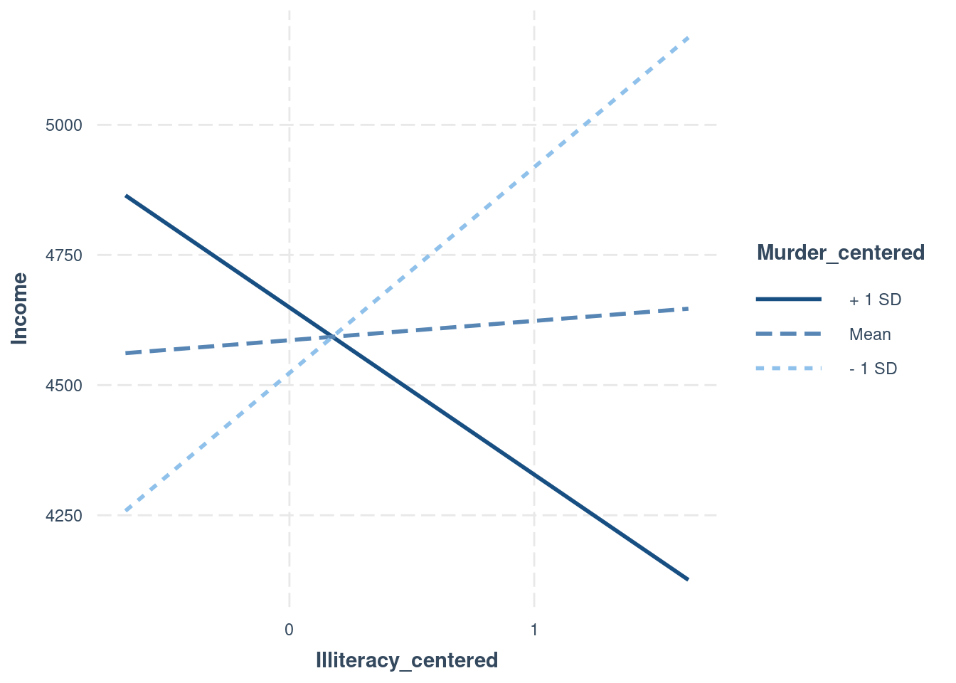
interactions::interact_plot(
  interactionModel,
  pred = Illiteracy_centered,
  modx = Murder_centered,
  plot.points = TRUE)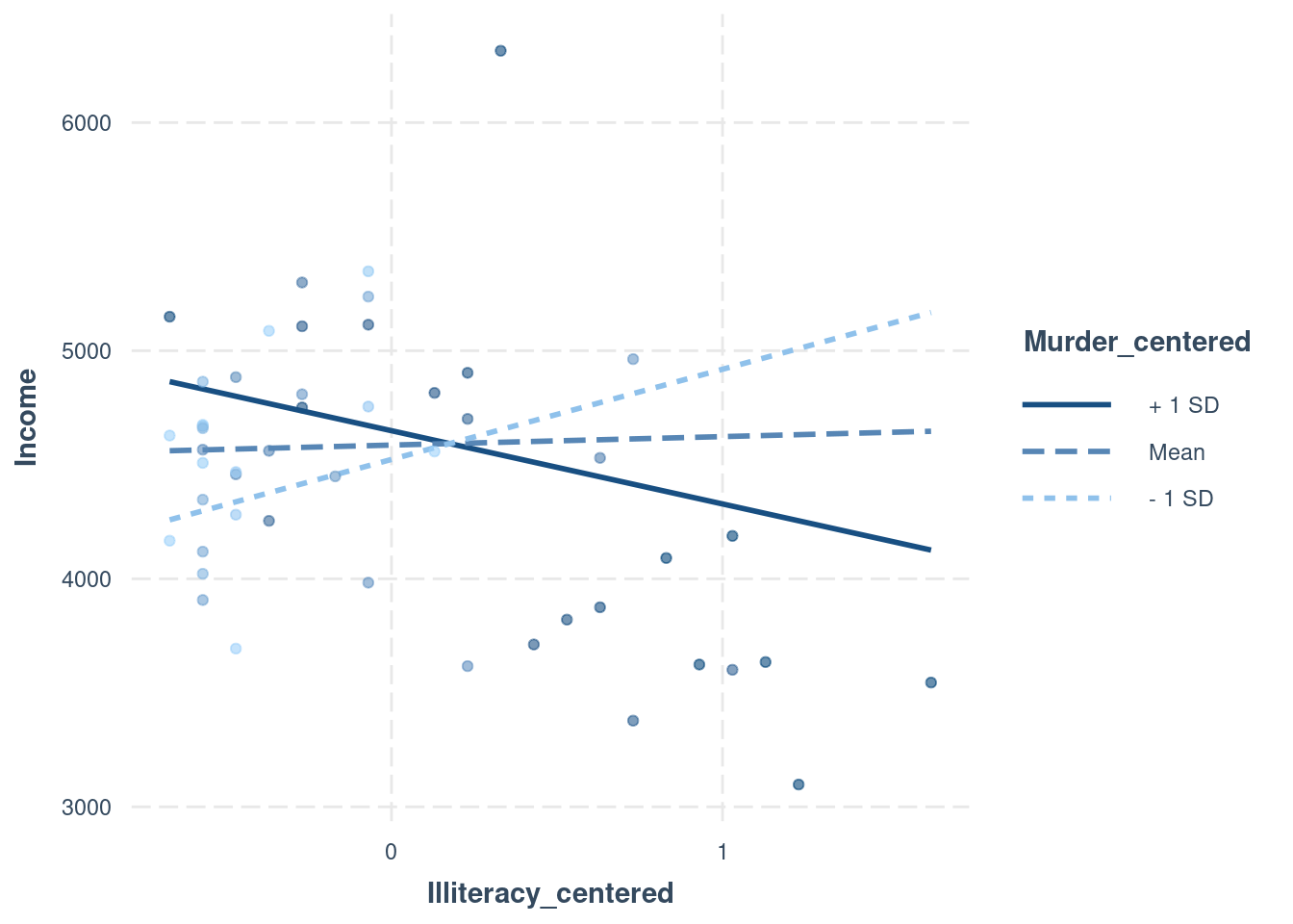
interactions::interact_plot(
  interactionModel,
  pred = Illiteracy_centered,
  modx = Murder_centered,
  interval = TRUE)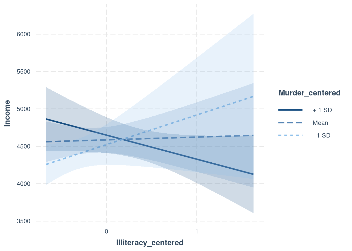
interactions::johnson_neyman(
  interactionModel,
  pred = Illiteracy_centered,
  modx = Murder_centered,
  alpha = .05)
JOHNSON-NEYMAN INTERVAL
When Murder_centered is OUTSIDE the interval [-8.13, 4.37], the slope of
Illiteracy_centered is p < .05.
Note: The range of observed values of Murder_centered is [-5.98, 7.72]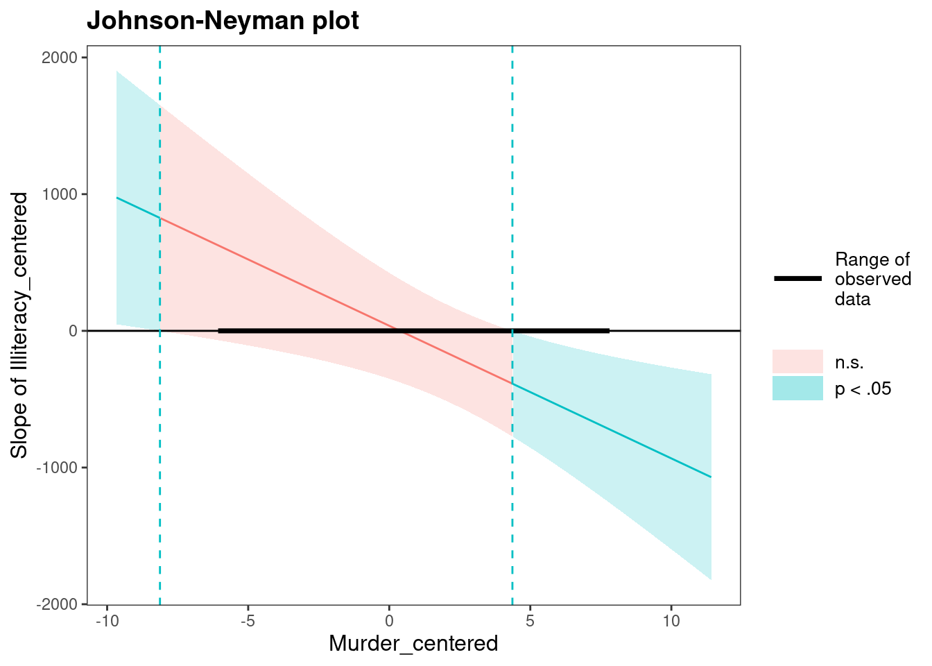
interactions::sim_slopes(
  interactionModel,
  pred = Illiteracy_centered,
  modx = Murder_centered,
  johnson_neyman = FALSE)
SIMPLE SLOPES ANALYSIS
Slope of Illiteracy_centered when Murder_centered = -3.69154e+00 (- 1 SD):
Est. S.E. t val. p
-------- -------- -------- ------
395.34 274.84 1.44 0.16
Slope of Illiteracy_centered when Murder_centered = -1.24345e-16 (Mean):
Est. S.E. t val. p
------- -------- -------- ------
37.12 192.56 0.19 0.85
Slope of Illiteracy_centered when Murder_centered = 3.69154e+00 (+ 1 SD):
Est. S.E. t val. p
--------- -------- -------- ------
-321.10 183.49 -1.75 0.09interactions::sim_slopes(
interactionModel,
pred = Illiteracy_centered,
modx = Murder_centered,
modx.values = c(0, 5, 10),
johnson_neyman = FALSE)SIMPLE SLOPES ANALYSIS
Slope of Illiteracy_centered when Murder_centered = 0.00:
Est. S.E. t val. p
------- -------- -------- ------
37.12 192.56 0.19 0.85
Slope of Illiteracy_centered when Murder_centered = 5.00:
Est. S.E. t val. p
--------- -------- -------- ------
-448.07 202.17 -2.22 0.03
Slope of Illiteracy_centered when Murder_centered = 10.00:
Est. S.E. t val. p
--------- -------- -------- ------
-933.27 330.10 -2.83 0.01Indicates all the values of the moderator for which the slope of the predictor is statistically significant.
interactions::sim_slopes(
interactionModel,
pred = Illiteracy_centered,
modx = Murder_centered,
johnson_neyman = TRUE)JOHNSON-NEYMAN INTERVAL
When Murder_centered is OUTSIDE the interval [-8.13, 4.37], the slope of
Illiteracy_centered is p < .05.
Note: The range of observed values of Murder_centered is [-5.98, 7.72]
SIMPLE SLOPES ANALYSIS

Slope of Illiteracy_centered when Murder_centered = -3.69154e+00 (- 1 SD):

    Est.     S.E.   t val.      p
-------- -------- -------- ------
  395.34   274.84     1.44   0.16

Slope of Illiteracy_centered when Murder_centered = -1.24345e-16 (Mean):

   Est.     S.E.   t val.      p
------- -------- -------- ------
  37.12   192.56     0.19   0.85

Slope of Illiteracy_centered when Murder_centered =  3.69154e+00 (+ 1 SD):

     Est.     S.E.   t val.      p
--------- -------- -------- ------
-321.10 183.49 -1.75 0.09interactions::probe_interaction(
interactionModel,
pred = Illiteracy_centered,
modx = Murder_centered,
cond.int = TRUE,
interval = TRUE,
jnplot = TRUE)JOHNSON-NEYMAN INTERVAL
When Murder_centered is OUTSIDE the interval [-8.13, 4.37], the slope of
Illiteracy_centered is p < .05.
Note: The range of observed values of Murder_centered is [-5.98, 7.72]
SIMPLE SLOPES ANALYSIS

When Murder_centered = -3.69154e+00 (- 1 SD):

                                        Est.     S.E.   t val.      p
---------------------------------- --------- -------- -------- ------
Slope of Illiteracy_centered          395.34   274.84     1.44   0.16
Conditional intercept                4523.23   134.99    33.51   0.00

When Murder_centered = -1.24345e-16 (Mean):

                                        Est.     S.E.   t val.      p
---------------------------------- --------- -------- -------- ------
Slope of Illiteracy_centered           37.12   192.56     0.19   0.85
Conditional intercept                4586.22    85.52    53.63   0.00

When Murder_centered =  3.69154e+00 (+ 1 SD):

                                        Est.     S.E.   t val.      p
---------------------------------- --------- -------- -------- ------
Slope of Illiteracy_centered         -321.10   183.49    -1.75   0.09
Conditional intercept                4649.22   118.97    39.08   0.00
Fisher’s r-to-z test.
http://comparingcorrelations.org (archived at https://perma.cc/X3EU-24GL)
Independent groups (two different groups):
cocor::cocor.indep.groups(
  r1.jk = .7,
  r2.hm = .6,
  n1 = 305,
  n2 = 210,
  data.name = c("group1", "group2"),
  var.labels = c("age", "intelligence", "age", "intelligence"))
  Results of a comparison of two correlations based on independent groups

Comparison between r1.jk (age, intelligence) = 0.7 and r2.hm (age, intelligence) = 0.6
Difference: r1.jk - r2.hm = 0.1
Data: group1: j = age, k = intelligence; group2: h = age, m = intelligence
Group sizes: n1 = 305, n2 = 210
Null hypothesis: r1.jk is equal to r2.hm
Alternative hypothesis: r1.jk is not equal to r2.hm (two-sided)
Alpha: 0.05

fisher1925: Fisher's z (1925)
  z = 1.9300, p-value = 0.0536
  Null hypothesis retained

zou2007: Zou's (2007) confidence interval
  95% confidence interval for r1.jk - r2.hm: -0.0014 0.2082
  Null hypothesis retained (Interval includes 0)
Dependent groups (same group), overlapping correlation (shares a variable in common—in this case, the variable age is shared in both correlations):
cocor::cocor.dep.groups.overlap(
  r.jk = .2, # Correlation (age, intelligence)
  r.jh = .5, # Correlation (age, shoe size)
  r.kh = .1, # Correlation (intelligence, shoe index)
  n = 315,
  var.labels = c("age", "intelligence", "shoe size"))
  Results of a comparison of two overlapping correlations based on dependent groups

Comparison between r.jk (age, intelligence) = 0.2 and r.jh (age, shoe size) = 0.5
Difference: r.jk - r.jh = -0.3
Related correlation: r.kh = 0.1
Data: j = age, k = intelligence, h = shoe size
Group size: n = 315
Null hypothesis: r.jk is equal to r.jh
Alternative hypothesis: r.jk is not equal to r.jh (two-sided)
Alpha: 0.05

pearson1898: Pearson and Filon's z (1898)
  z = -4.4807, p-value = 0.0000
  Null hypothesis rejected

hotelling1940: Hotelling's t (1940)
  t = -4.6314, df = 312, p-value = 0.0000
  Null hypothesis rejected

williams1959: Williams' t (1959)
  t = -4.4950, df = 312, p-value = 0.0000
  Null hypothesis rejected

olkin1967: Olkin's z (1967)
  z = -4.4807, p-value = 0.0000
  Null hypothesis rejected

dunn1969: Dunn and Clark's z (1969)
  z = -4.4412, p-value = 0.0000
  Null hypothesis rejected

hendrickson1970: Hendrickson, Stanley, and Hills' (1970) modification of Williams' t (1959)
  t = -4.6313, df = 312, p-value = 0.0000
  Null hypothesis rejected

steiger1980: Steiger's (1980) modification of Dunn and Clark's z (1969) using average correlations
  z = -4.4152, p-value = 0.0000
  Null hypothesis rejected

meng1992: Meng, Rosenthal, and Rubin's z (1992)
  z = -4.3899, p-value = 0.0000
  Null hypothesis rejected
  95% confidence interval for r.jk - r.jh: -0.5013 -0.1918
  Null hypothesis rejected (Interval does not include 0)

hittner2003: Hittner, May, and Silver's (2003) modification of Dunn and Clark's z (1969) using a backtransformed average Fisher's (1921) Z procedure
  z = -4.4077, p-value = 0.0000
  Null hypothesis rejected

zou2007: Zou's (2007) confidence interval
  95% confidence interval for r.jk - r.jh: -0.4307 -0.1675
  Null hypothesis rejected (Interval does not include 0)
Dependent groups (same group), non-overlapping correlation (does not share a variable in common):
cocor::cocor.dep.groups.nonoverlap(
  r.jk = .2, # Correlation (age, intelligence)
  r.hm = .7, # Correlation (body mass index, shoe size)
  r.jh = .4, # Correlation (age, body mass index)
  r.jm = .5, # Correlation (age, shoe size)
  r.kh = .1, # Correlation (intelligence, body mass index)
  r.km = .3, # Correlation (intelligence, shoe size)
  n = 232,
  var.labels = c("age", "intelligence", "body mass index", "shoe size"))
  Results of a comparison of two nonoverlapping correlations based on dependent groups

Comparison between r.jk (age, intelligence) = 0.2 and r.hm (body mass index, shoe size) = 0.7
Difference: r.jk - r.hm = -0.5
Related correlations: r.jh = 0.4, r.jm = 0.5, r.kh = 0.1, r.km = 0.3
Data: j = age, k = intelligence, h = body mass index, m = shoe size
Group size: n = 232
Null hypothesis: r.jk is equal to r.hm
Alternative hypothesis: r.jk is not equal to r.hm (two-sided)
Alpha: 0.05

pearson1898: Pearson and Filon's z (1898)
  z = -7.1697, p-value = 0.0000
  Null hypothesis rejected

dunn1969: Dunn and Clark's z (1969)
  z = -7.3134, p-value = 0.0000
  Null hypothesis rejected

steiger1980: Steiger's (1980) modification of Dunn and Clark's z (1969) using average correlations
  z = -7.3010, p-value = 0.0000
  Null hypothesis rejected

raghunathan1996: Raghunathan, Rosenthal, and Rubin's (1996) modification of Pearson and Filon's z (1898)
  z = -7.3134, p-value = 0.0000
  Null hypothesis rejected

silver2004: Silver, Hittner, and May's (2004) modification of Dunn and Clark's z (1969) using a backtransformed average Fisher's (1921) Z procedure
  z = -7.2737, p-value = 0.0000
  Null hypothesis rejected

zou2007: Zou's (2007) confidence interval
  95% confidence interval for r.jk - r.hm: -0.6375 -0.3629
Null hypothesis rejected (Interval does not include 0)Listwise deletion deletes every row in the data file that has a missing value for one of the model variables.
Call:
lm(formula = bpi_antisocialT2Sum ~ bpi_antisocialT1Sum + bpi_anxiousDepressedSum,
    data = mydata, na.action = na.exclude)

Residuals:
    Min      1Q  Median      3Q     Max
-8.3755 -1.2337 -0.2212  0.9911 12.8017

Coefficients:
                        Estimate Std. Error t value Pr(>|t|)
(Intercept)              1.19830    0.05983  20.029  < 2e-16 ***
bpi_antisocialT1Sum      0.46553    0.01858  25.049  < 2e-16 ***
bpi_anxiousDepressedSum  0.16075    0.02916   5.513 3.83e-08 ***
---
Signif. codes:  0 '***' 0.001 '**' 0.01 '*' 0.05 '.' 0.1 ' ' 1

Residual standard error: 1.979 on 2871 degrees of freedom
  (8656 observations deleted due to missingness)
Multiple R-squared:  0.262, Adjusted R-squared:  0.2615
F-statistic: 509.6 on 2 and 2871 DF, p-value: < 2.2e-16confint(listwiseDeletionModel) 2.5 % 97.5 %
(Intercept) 1.0809881 1.3156128
bpi_antisocialT1Sum 0.4290884 0.5019688
bpi_anxiousDepressedSum 0.1035825 0.2179258print(effectsize::standardize_parameters(listwiseDeletionModel), digits = 2)# Standardization method: refit
Parameter | Std. Coef. | 95% CI
----------------------------------------------------
(Intercept) | 1.62e-16 | [-0.03, 0.03]
bpi antisocialT1Sum | 0.46 | [ 0.42, 0.49]
bpi anxiousDepressedSum | 0.10 | [ 0.06, 0.14]Also see here:
Adapted from here: https://stefvanbuuren.name/fimd/sec-simplesolutions.html#sec:pairwise (archived at https://perma.cc/EGU6-3M3Q)
modelData <- mydata[,c("bpi_antisocialT2Sum","bpi_antisocialT1Sum","bpi_anxiousDepressedSum")]
varMeans <- colMeans(modelData, na.rm = TRUE)
varCovariances <- cov(modelData, use = "pairwise")

pairwiseRegression_syntax <- '
  bpi_antisocialT2Sum ~ bpi_antisocialT1Sum + bpi_anxiousDepressedSum
  bpi_antisocialT2Sum ~~ bpi_antisocialT2Sum
  bpi_antisocialT2Sum ~ 1
'

pairwiseRegression_fit <- lavaan::lavaan(
  pairwiseRegression_syntax,
  sample.mean = varMeans,
  sample.cov = varCovariances,
  sample.nobs = sum(complete.cases(modelData))
)

summary(
  pairwiseRegression_fit,
  standardized = TRUE,
  rsquare = TRUE)
lavaan 0.7-2 ended normally after 1 iteration
Estimator ML
Optimization method NLMINB
Number of model parameters 4
Number of observations 2874
Model Test User Model:
Test statistic 0.000
Degrees of freedom 0
Parameter Estimates:
Standard errors Standard
Information Expected
Information saturated (h1) model Structured
Regressions:
Estimate Std.Err z-value P(>|z|) Std.lv Std.all
bpi_antisocialT2Sum ~
bpi_antsclT1Sm 0.441 0.018 24.611 0.000 0.441 0.456
bp_nxsDprssdSm 0.137 0.028 4.854 0.000 0.137 0.090
Intercepts:
Estimate Std.Err z-value P(>|z|) Std.lv Std.all
.bpi_antsclT2Sm 1.175 0.058 20.125 0.000 1.175 0.523
Variances:
Estimate Std.Err z-value P(>|z|) Std.lv Std.all
.bpi_antsclT2Sm 3.755 0.099 37.908 0.000 3.755 0.743
R-Square:
Estimate
bpi_antsclT2Sm 0.257fimlRegression_syntax <- '
bpi_antisocialT2Sum ~ bpi_antisocialT1Sum + bpi_anxiousDepressedSum
bpi_antisocialT2Sum ~~ bpi_antisocialT2Sum
bpi_antisocialT2Sum ~ 1
'
fimlRegression_fit <- lavaan::lavaan(
fimlRegression_syntax,
data = mydata,
missing = "ML",
)
summary(
fimlRegression_fit,
standardized = TRUE,
rsquare = TRUE)lavaan 0.7-2 ended normally after 11 iterations
Estimator ML
Optimization method NLMINB
Number of model parameters 4
Used Total
Number of observations 3914 11530
Number of missing patterns 2
Model Test User Model:
Test statistic 0.000
Degrees of freedom 0
Parameter Estimates:
Standard errors Standard
Information Observed
Observed information based on Hessian
Regressions:
Estimate Std.Err z-value P(>|z|) Std.lv Std.all
bpi_antisocialT2Sum ~
bpi_antsclT1Sm 0.466 0.019 25.062 0.000 0.466 0.466
bp_nxsDprssdSm 0.161 0.029 5.516 0.000 0.161 0.102
Intercepts:
Estimate Std.Err z-value P(>|z|) Std.lv Std.all
.bpi_antsclT2Sm 1.198 0.060 20.039 0.000 1.198 0.516
Variances:
Estimate Std.Err z-value P(>|z|) Std.lv Std.all
.bpi_antsclT2Sm 3.911 0.103 37.908 0.000 3.911 0.725
R-Square:
Estimate
bpi_antsclT2Sm 0.275modelData_imputed <- mice::mice(
modelData,
m = 5,
method = "pmm") # predictive mean matching; can choose among many methods
 iter imp variable
  1   1  bpi_antisocialT2Sum  bpi_antisocialT1Sum  bpi_anxiousDepressedSum
  1   2  bpi_antisocialT2Sum  bpi_antisocialT1Sum  bpi_anxiousDepressedSum
  1   3  bpi_antisocialT2Sum  bpi_antisocialT1Sum  bpi_anxiousDepressedSum
  1   4  bpi_antisocialT2Sum  bpi_antisocialT1Sum  bpi_anxiousDepressedSum
  1   5  bpi_antisocialT2Sum  bpi_antisocialT1Sum  bpi_anxiousDepressedSum
  2   1  bpi_antisocialT2Sum  bpi_antisocialT1Sum  bpi_anxiousDepressedSum
  2   2  bpi_antisocialT2Sum  bpi_antisocialT1Sum  bpi_anxiousDepressedSum
  2   3  bpi_antisocialT2Sum  bpi_antisocialT1Sum  bpi_anxiousDepressedSum
  2   4  bpi_antisocialT2Sum  bpi_antisocialT1Sum  bpi_anxiousDepressedSum
  2   5  bpi_antisocialT2Sum  bpi_antisocialT1Sum  bpi_anxiousDepressedSum
  3   1  bpi_antisocialT2Sum  bpi_antisocialT1Sum  bpi_anxiousDepressedSum
  3   2  bpi_antisocialT2Sum  bpi_antisocialT1Sum  bpi_anxiousDepressedSum
  3   3  bpi_antisocialT2Sum  bpi_antisocialT1Sum  bpi_anxiousDepressedSum
  3   4  bpi_antisocialT2Sum  bpi_antisocialT1Sum  bpi_anxiousDepressedSum
  3   5  bpi_antisocialT2Sum  bpi_antisocialT1Sum  bpi_anxiousDepressedSum
  4   1  bpi_antisocialT2Sum  bpi_antisocialT1Sum  bpi_anxiousDepressedSum
  4   2  bpi_antisocialT2Sum  bpi_antisocialT1Sum  bpi_anxiousDepressedSum
  4   3  bpi_antisocialT2Sum  bpi_antisocialT1Sum  bpi_anxiousDepressedSum
  4   4  bpi_antisocialT2Sum  bpi_antisocialT1Sum  bpi_anxiousDepressedSum
  4   5  bpi_antisocialT2Sum  bpi_antisocialT1Sum  bpi_anxiousDepressedSum
  5   1  bpi_antisocialT2Sum  bpi_antisocialT1Sum  bpi_anxiousDepressedSum
  5   2  bpi_antisocialT2Sum  bpi_antisocialT1Sum  bpi_anxiousDepressedSum
  5   3  bpi_antisocialT2Sum  bpi_antisocialT1Sum  bpi_anxiousDepressedSum
  5   4  bpi_antisocialT2Sum  bpi_antisocialT1Sum  bpi_anxiousDepressedSum
5 5 bpi_antisocialT2Sum bpi_antisocialT1Sum bpi_anxiousDepressedSumrockchalk::getDeltaRsquare(multipleRegressionModel)The deltaR-square values: the change in the R-square
observed when a single term is removed.
Same as the square of the 'semi-partial correlation coefficient'
deltaRsquare
bpi_antisocialT1Sum 0.161297120
bpi_anxiousDepressedSum 0.007813728A partial regression plot (aka added-variable) examines the association between the predictor and the outcome after controlling for the covariates.
car::avPlots(
  multipleRegressionModel,
  id = FALSE)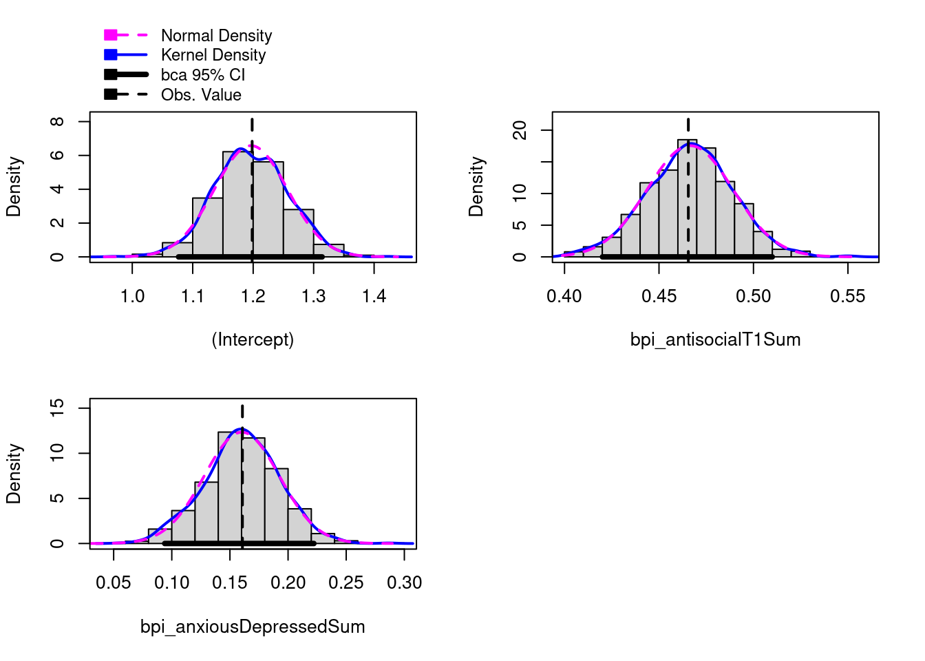
Manually:
# DV residuals (outcome residualized on covariates)
ry <- resid(lm(
  bpi_antisocialT2Sum ~ bpi_antisocialT1Sum,
  data = mydata, na.action = na.exclude))

# Predictor residuals (focal predictor residualized on covariates)
rx <- resid(lm(
  bpi_anxiousDepressedSum ~ bpi_antisocialT1Sum,
  data = mydata, na.action = na.exclude))

# Create the partial regression plot
df_plot <- data.frame(rx, ry)

ggplot(
  data = df_plot,
  mapping = aes(x = rx, y = ry)) +
  geom_point(alpha = 0.6) +
  geom_smooth(
    method = "lm",
    color = "blue") +
  labs(
    x = "Residualized bpi_antisocialT1Sum",
    y = "Residualized bpi_antisocialT2Sum",
    title = "Partial Regression Plot\nbpi_antisocialT2Sum ~ bpi_antisocialT1Sum controlling for bpi_anxiousDepressedSum"
  )
parameters::dominance_analysis(multipleRegressionModel)# Dominance Analysis Results
Model R2 Value: 0.262
General Dominance Statistics
Parameter | General Dominance | Percent | Ranks | Subset
---------------------------------------------------------------------------------------
(Intercept) | | | | constant
bpi_antisocialT1Sum | 0.208 | 0.793 | 1 | bpi_antisocialT1Sum
bpi_anxiousDepressedSum | 0.054 | 0.207 | 2 | bpi_anxiousDepressedSum
Conditional Dominance Statistics
Subset | IVs: 1 | IVs: 2
-----------------------------------------
bpi_antisocialT1Sum | 0.254 | 0.161
bpi_anxiousDepressedSum | 0.101 | 0.008
Complete Dominance Designations
Subset | < bpi_antisocialT1Sum | < bpi_anxiousDepressedSum
---------------------------------------------------------------------------
bpi_antisocialT1Sum | | FALSE
bpi_anxiousDepressedSum | TRUE | $DA
k R2 bpi_antisocialT1Sum.Inc
bpi_antisocialT1Sum 1 0.2541698 NA
bpi_anxiousDepressedSum 1 0.1006864 0.1612971
bpi_antisocialT1Sum,bpi_anxiousDepressedSum 2 0.2619835 NA
bpi_anxiousDepressedSum.Inc
bpi_antisocialT1Sum 0.007813728
bpi_anxiousDepressedSum NA
bpi_antisocialT1Sum,bpi_anxiousDepressedSum NA
$CD
bpi_antisocialT1Sum bpi_anxiousDepressedSum
CD:0 0.2541698 0.100686422
CD:1 0.1612971 0.007813728
$GD
bpi_antisocialT1Sum bpi_anxiousDepressedSum
0.20773347 0.05425008 yhat::calc.yhat(multipleRegressionModel)$PredictorMetrics
b Beta r rs rs2 Unique Common CD:0 CD:1
bpi_antisocialT1Sum 0.466 0.456 0.504 0.985 0.970 0.161 0.093 0.254 0.161
bpi_anxiousDepressedSum 0.161 0.100 0.317 0.620 0.384 0.008 0.093 0.101 0.008
Total NA NA NA NA 1.354 0.169 0.186 0.355 0.169
GenDom Pratt RLW
bpi_antisocialT1Sum 0.208 0.230 0.208
bpi_anxiousDepressedSum 0.054 0.032 0.054
Total 0.262 0.262 0.262
$OrderedPredictorMetrics
b Beta r rs rs2 Unique Common CD:0 CD:1 GenDom Pratt
bpi_antisocialT1Sum 1 1 1 1 1 1 1 1 1 1 1
bpi_anxiousDepressedSum 2 2 2 2 2 2 2 2 2 2 2
RLW
bpi_antisocialT1Sum 1
bpi_anxiousDepressedSum 2
$PairedDominanceMetrics
Comp Cond Gen
bpi_antisocialT1Sum>bpi_anxiousDepressedSum 1 1 1
$APSRelatedMetrics
Commonality % Total R2
bpi_antisocialT1Sum 0.161 0.616 0.254
bpi_anxiousDepressedSum 0.008 0.030 0.101
bpi_antisocialT1Sum,bpi_anxiousDepressedSum 0.093 0.354 0.262
Total 0.262 1.000 NA
bpi_antisocialT1Sum.Inc
bpi_antisocialT1Sum NA
bpi_anxiousDepressedSum 0.161
bpi_antisocialT1Sum,bpi_anxiousDepressedSum NA
Total NA
bpi_anxiousDepressedSum.Inc
bpi_antisocialT1Sum 0.008
bpi_anxiousDepressedSum NA
bpi_antisocialT1Sum,bpi_anxiousDepressedSum NA
Total NAallPossibleSubsetsRegression <- yhat::aps(
dataMatrix = mydata,
dv = "bpi_antisocialT2Sum",
ivlist = list("bpi_antisocialT1Sum", "bpi_anxiousDepressedSum"))
yhat::commonality(allPossibleSubsetsRegression) Coefficient % Total
bpi_antisocialT1Sum 0.161297120 0.61567654
bpi_anxiousDepressedSum 0.007813728 0.02982526
bpi_antisocialT1Sum,bpi_anxiousDepressedSum 0.092872694 0.35449820commonalityAnalysis <- yhat::commonalityCoefficients(
dataMatrix = mydata,
dv = "bpi_antisocialT2Sum",
ivlist = list("bpi_antisocialT1Sum", "bpi_anxiousDepressedSum"))
commonalityAnalysis$CC
Coefficient
Unique to bpi_antisocialT1Sum 0.1613
Unique to bpi_anxiousDepressedSum 0.0078
Common to bpi_antisocialT1Sum, and bpi_anxiousDepressedSum 0.0929
Total 0.2620
% Total
Unique to bpi_antisocialT1Sum 61.57
Unique to bpi_anxiousDepressedSum 2.98
Common to bpi_antisocialT1Sum, and bpi_anxiousDepressedSum 35.45
Total 100.00
$CCTotalbyVar
Unique Common Total
bpi_antisocialT1Sum 0.1613 0.0929 0.2542
bpi_anxiousDepressedSum 0.0078 0.0929 0.1007mcar_test() function of the njtierney/naniar packageTo determine the confidence intervals of parameter estimates
multipleRegressionModelBootstrapped <- Boot(multipleRegressionModelNoMissing, R = 1000)Error:
! object 'multipleRegressionModelNoMissing' not foundsummary(multipleRegressionModelBootstrapped)Error in `h()`:
! error in evaluating the argument 'object' in selecting a method for function 'summary': object 'multipleRegressionModelBootstrapped' not foundconfint(multipleRegressionModelBootstrapped, level = .95, type = "bca")Error:
! object 'multipleRegressionModelBootstrapped' not foundhist(multipleRegressionModelBootstrapped)Error:
! object 'multipleRegressionModelBootstrapped' not foundgeneralizedRegressionModelBootstrapped <- Boot(multipleRegressionModelNoMissing, R = 1000)Error:
! object 'multipleRegressionModelNoMissing' not foundsummary(generalizedRegressionModelBootstrapped)Error in `h()`:
! error in evaluating the argument 'object' in selecting a method for function 'summary': object 'generalizedRegressionModelBootstrapped' not foundconfint(generalizedRegressionModelBootstrapped, level = .95, type = "bca")Error:
! object 'generalizedRegressionModelBootstrapped' not foundhist(generalizedRegressionModelBootstrapped)Error:
! object 'generalizedRegressionModelBootstrapped' not foundTo examine degree of prediction error and over-fitting to determine best model
https://stats.stackexchange.com/questions/103459/how-do-i-know-which-method-of-cross-validation-is-best (archived at https://perma.cc/38BL-KLRJ)
kFolds <- 10
replications <- 20
folds <- cvFolds(nrow(mydata), K = kFolds, R = replications)
fitLm <- lm(
bpi_antisocialT2Sum ~ bpi_antisocialT1Sum + bpi_anxiousDepressedSum,
data = mydata,
na.action = "na.exclude")
fitLmrob <- lmrob(
bpi_antisocialT2Sum ~ bpi_antisocialT1Sum + bpi_anxiousDepressedSum,
data = mydata,
na.action = "na.exclude")
fitLts <- ltsReg(
bpi_antisocialT2Sum ~ bpi_antisocialT1Sum + bpi_anxiousDepressedSum,
data = mydata,
na.action = "na.exclude")
cvFitLm <- cvLm(
fitLm,
K = kFolds,
R = replications)
cvFitLmrob <- cvLmrob(
fitLmrob,
K = kFolds,
R = replications)
cvFitLts <- cvLts(
fitLts,
K = kFolds,
R = replications)
cvFits <- cvSelect(
OLS = cvFitLm,
MM = cvFitLmrob,
LTS = cvFitLts)
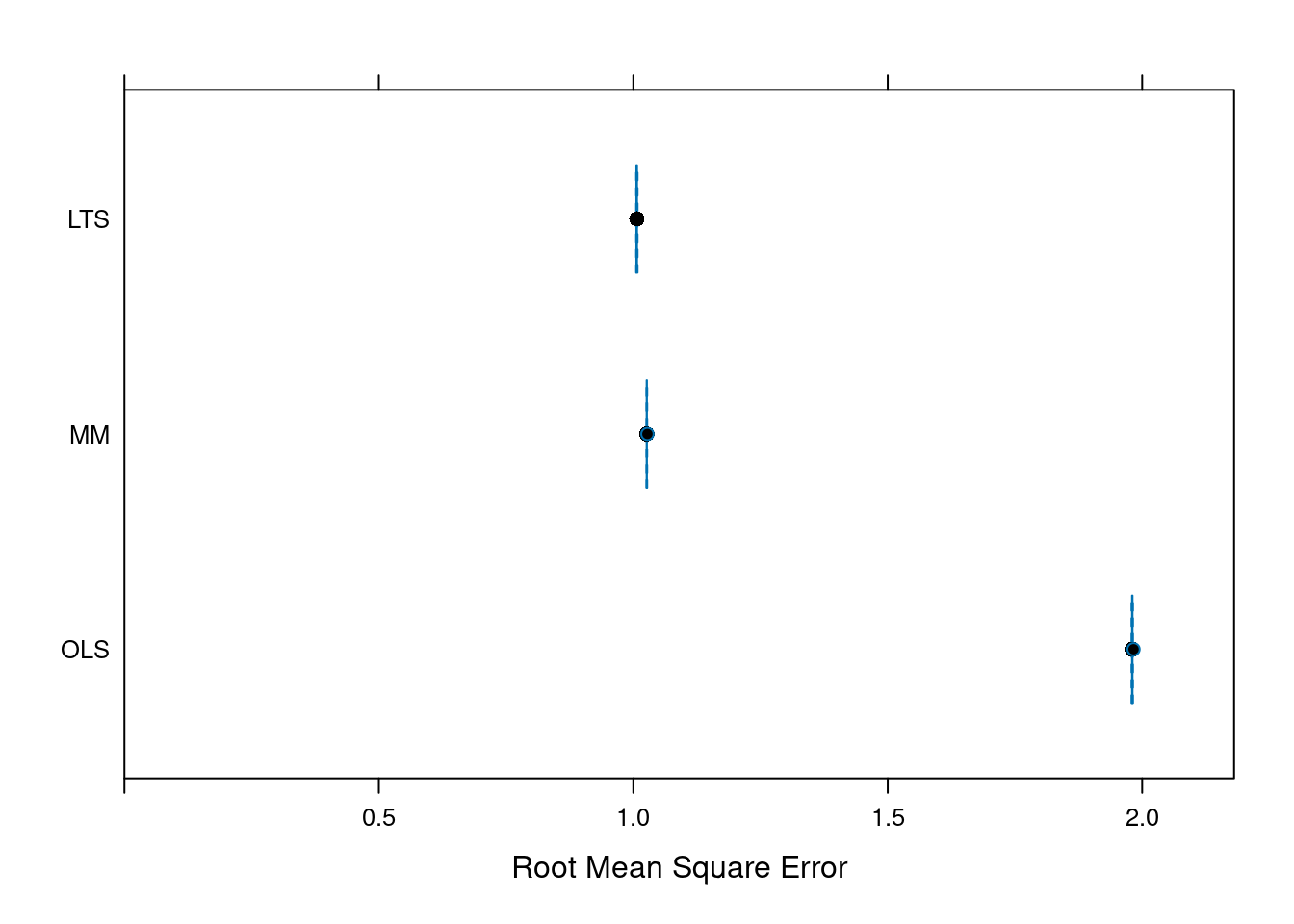
cvFits
10-fold CV results:
  Fit       CV
1 OLS 1.980506
2  MM 1.026593
3 LTS 1.007115

Best model:
   CV
"LTS" 
allEffects(multipleRegressionModel) model: bpi_antisocialT2Sum ~ bpi_antisocialT1Sum + bpi_anxiousDepressedSum
bpi_antisocialT1Sum effect
bpi_antisocialT1Sum
0 3.2 6.5 9.8 13
1.394591 2.884283 4.420527 5.956772 7.446463
bpi_anxiousDepressedSum effect
bpi_anxiousDepressedSum
0 2 4 6 8
2.502636 2.824145 3.145653 3.467161 3.788669 plot(allEffects(multipleRegressionModel))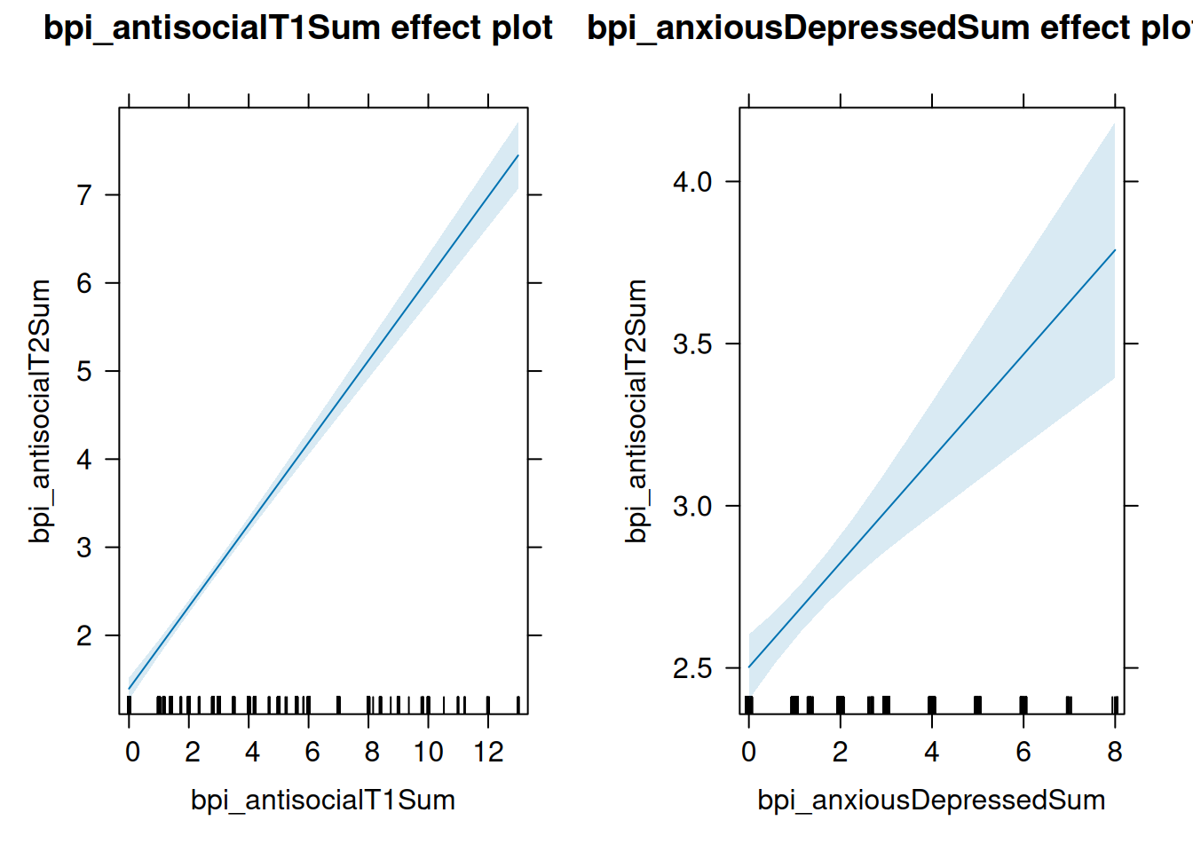
confidenceEllipse(
  multipleRegressionModel,
  levels = c(0.5, .95))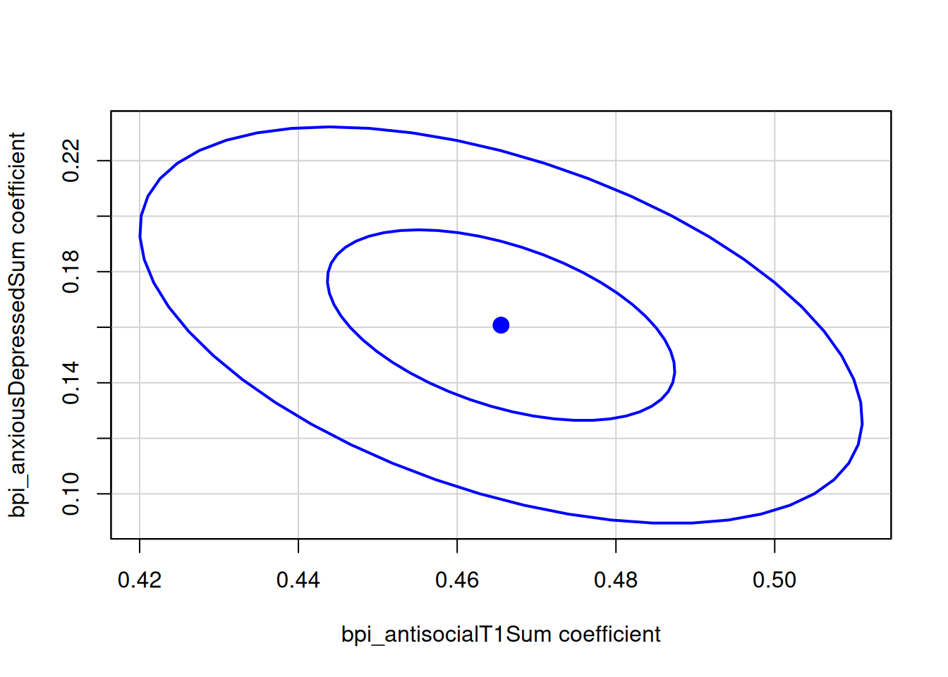
mydata_nomissing <- na.omit(mydata[,c("bpi_antisocialT1Sum","bpi_antisocialT2Sum")])
dataEllipse(
  mydata_nomissing$bpi_antisocialT1Sum,
  mydata_nomissing$bpi_antisocialT2Sum,
  levels = c(0.5, .95))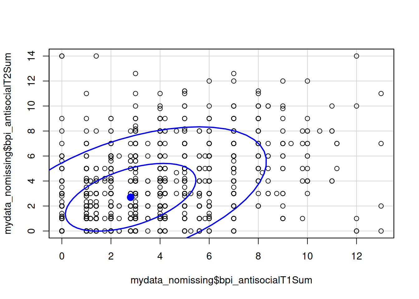
scatterplotMatrix(
  ~ bpi_antisocialT2Sum + bpi_antisocialT1Sum + bpi_anxiousDepressedSum,
  data = mydata)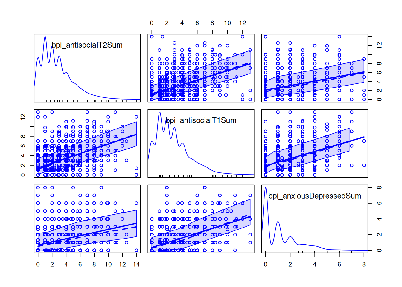
The distance correlation is an index of the degree of the linear and non-linear association between two variables.
correlation(
  mydata[,c("bpi_antisocialT1Sum","bpi_antisocialT2Sum")],
  method = "distance",
p_adjust = "none")Check for nonlinearities (non-horizontal line) in plots of:
http://www.lisa.stat.vt.edu/?q=node/7517 (archived at https://web.archive.org/web/20180113065042/http://www.lisa.stat.vt.edu/?q=node/7517)
Note: using semi-parametric or non-parametric models increases fit in context of nonlinearity at the expense of added complexity. Make sure to avoid fitting an overly complex model (e.g., use k-fold cross validation). Often, the simpler (generalized) linear model is preferable to semi-paremetric or non-parametric approaches
http://documents.software.dell.com/Statistics/Textbook/Generalized-Additive-Models (archived at https://web.archive.org/web/20170213041653/http://documents.software.dell.com/Statistics/Textbook/Generalized-Additive-Models)
Family: gaussian
Link function: identity

Formula:
bpi_antisocialT2Sum ~ bpi_antisocialT1Sum + bpi_anxiousDepressedSum

Parametric coefficients:
                        Estimate Std. Error t value Pr(>|t|)
(Intercept)              1.19830    0.05983  20.029  < 2e-16 ***
bpi_antisocialT1Sum      0.46553    0.01858  25.049  < 2e-16 ***
bpi_anxiousDepressedSum  0.16075    0.02916   5.513 3.83e-08 ***
---
Signif. codes:  0 '***' 0.001 '**' 0.01 '*' 0.05 '.' 0.1 ' ' 1


R-sq.(adj) =  0.261   Deviance explained = 26.2%
GCV = 3.9191 Scale est. = 3.915 n = 2874confint(generalizedAdditiveModel)Error in `glm.control()`:
! unused arguments (nthreads = 1, ncv.threads = 1, irls.reg = 0, mgcv.tol = 1e-07, mgcv.half = 15, rank.tol = 1.49011611938477e-08, nlm = list(7, 1e-06, 2, 1e-04, 200, FALSE), optim = list(1e+07), newton = list(1e-06, 5, 2, 30, FALSE), idLinksBases = TRUE, scalePenalty = TRUE, efs.lspmax = 15, efs.tol = 0.1, keepData = FALSE, scale.est = "fletcher", edge.correct = FALSE)Exogeneity means that the association between predictors and outcome is fully causal and unrelated to other variables.
The instrumental variables (2SLS) estimator is implemented in the R package AER as command:
ivreg(y ~ x1 + x2 + w1 + w2 | z1 + z2 + z3 + w1 + w2)where x1 and x2 are endogenous regressors, w1 and w2 exogeneous regressors, and z1 to z3 are excluded instruments.
Durbin-Wu-Hausman test:
hsng2 <- read.dta("https://www.stata-press.com/data/r11/hsng2.dta") #archived at https://perma.cc/7P2Q-ARKR
Call:
ivreg(formula = rent ~ hsngval + pcturban | pcturban + faminc +
    reg2 + reg3 + reg4, data = hsng2)

Residuals:
     Min       1Q   Median       3Q      Max
-84.1948 -11.6023  -0.5239   8.6583  73.6130

Coefficients:
             Estimate Std. Error t value Pr(>|t|)
(Intercept) 1.207e+02  1.571e+01   7.685 7.55e-10 ***
hsngval     2.240e-03  3.388e-04   6.612 3.17e-08 ***
pcturban    8.152e-02  3.082e-01   0.265    0.793

Diagnostic tests:
                 df1 df2 statistic  p-value
Weak instruments   4  44     13.30  3.5e-07 ***
Wu-Hausman         1  46     15.91 0.000236 ***
Sargan             3  NA     11.29 0.010268 *
---
Signif. codes:  0 '***' 0.001 '**' 0.01 '*' 0.05 '.' 0.1 ' ' 1

Residual standard error: 22.86 on 47 degrees of freedom
Multiple R-Squared: 0.5989, Adjusted R-squared: 0.5818
Wald test: 42.66 on 2 and 47 DF,  p-value: 2.731e-11
The Eicker-Huber-White covariance estimator which is robust to heteroscedastic error terms is reported after estimation with vcov = sandwich in coeftest()
First stage results are reported by explicitly estimating them. For example:
Call:
lm(formula = hsngval ~ pcturban + faminc + reg2 + reg3 + reg4,
    data = hsng2)

Residuals:
   Min     1Q Median     3Q    Max
-10504  -5223  -1162   2939  46756

Coefficients:
              Estimate Std. Error t value Pr(>|t|)
(Intercept) -1.867e+04  1.200e+04  -1.557 0.126736
pcturban     1.822e+02  1.150e+02   1.584 0.120289
faminc       2.731e+00  6.819e-01   4.006 0.000235 ***
reg2        -5.095e+03  4.122e+03  -1.236 0.223007
reg3        -1.778e+03  4.073e+03  -0.437 0.664552
reg4         1.341e+04  4.048e+03   3.314 0.001849 **
---
Signif. codes:  0 '***' 0.001 '**' 0.01 '*' 0.05 '.' 0.1 ' ' 1

Residual standard error: 9253 on 44 degrees of freedom
Multiple R-squared:  0.6908,    Adjusted R-squared:  0.6557
F-statistic: 19.66 on 5 and 44 DF,  p-value: 3.032e-10
In case of a single endogenous variable (K = 1), the F-statistic to assess weak instruments is reported after estimating the first stage with, for example:
waldtest(
  first,
  . ~ . - faminc - reg2 - reg3 - reg4)
or in case of heteroscedatistic errors:
waldtest(
  first,
  . ~ . - faminc - reg2 - reg3- reg4,
vcov = sandwich)Homoscedasticity of the residuals means that the variance of the residuals does not differ as a function of the outcome/predictors (i.e., the residuals show constant variance as a function of outcome/predictors).
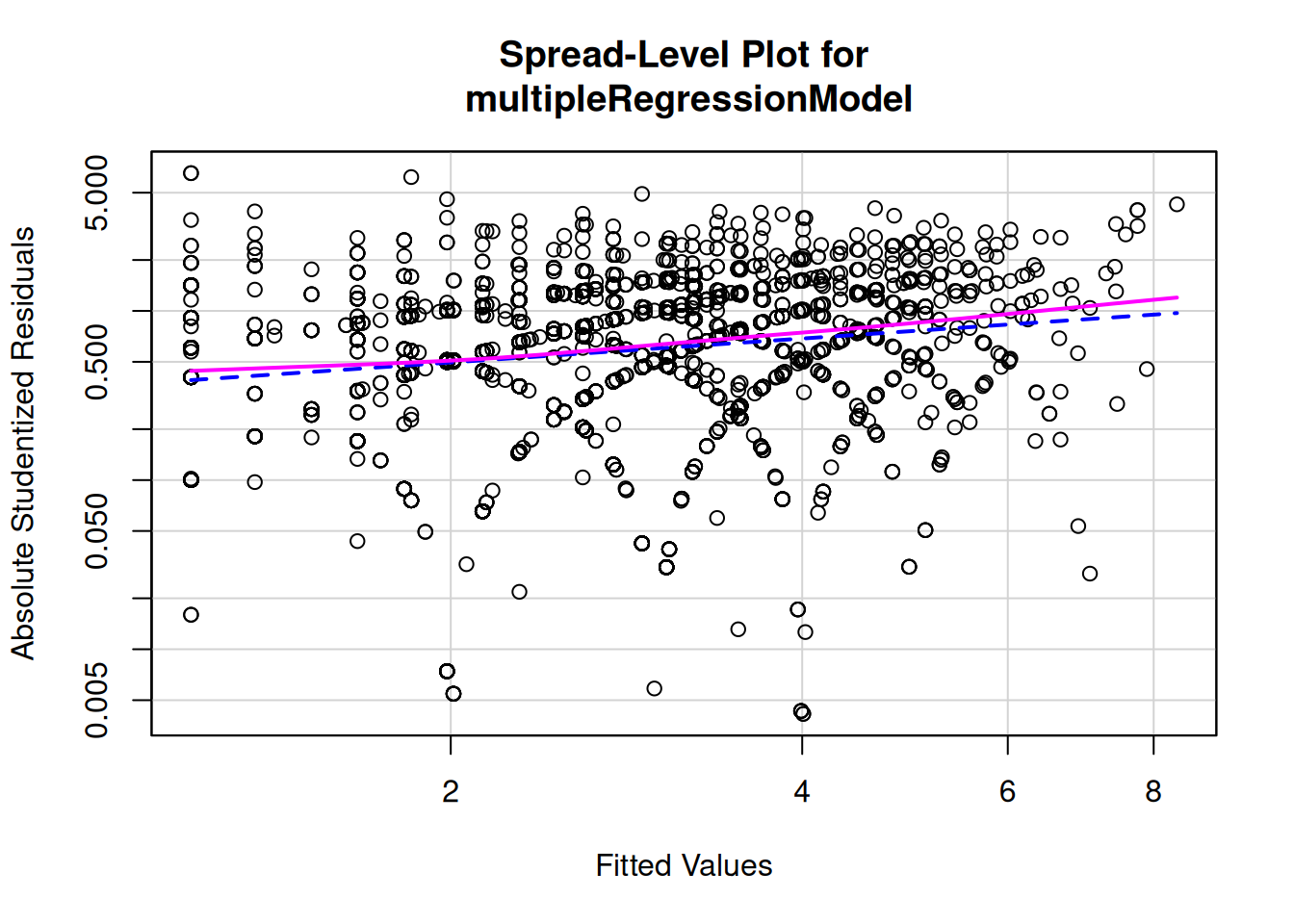
bptest() function from lmtest packagePlot residuals, or perhaps their absolute values, versus the outcome and predictor variables (Residual Plots). Examine whether residual variance is constant at all levels of other variables or whether it increases/decreases as a function of another variable (or shows some others structure, e.g., small variance at low and high levels of a predictor and high variance in the middle). Note that this is different than whether the residuals show non-linearities—i.e., a non-horizontal line, which would indicate a nonlinear association between variables (see Assumption #1, above). Rather, here we are examining whether there is change in the variance as a function of another variable (e.g., a fan-shaped Residual Plot)
Examining whether level (e.g., mean) depends on spread (e.g., variance)—plot of log of the absolute Studentized residuals against the log of the fitted values
https://www.rdocumentation.org/packages/lmtest/versions/0.9-40/topics/bptest (archived at https://perma.cc/K4WC-7TVW)
bptest(multipleRegressionModel)
    studentized Breusch-Pagan test

data:  multipleRegressionModel
BP = 94.638, df = 2, p-value < 2.2e-16gqtest(multipleRegressionModel)
    Goldfeld-Quandt test

data:  multipleRegressionModel
GQ = 1.0755, df1 = 1434, df2 = 1434, p-value = 0.08417
alternative hypothesis: variance increases from segment 1 to 2ncvTest(multipleRegressionModel)Non-constant Variance Score Test
Variance formula: ~ fitted.values
Chisquare = 232.1196, Df = 1, p = < 2.22e-16ncvTest(
multipleRegressionModel,
~ bpi_antisocialT1Sum + bpi_anxiousDepressedSum)Non-constant Variance Score Test
Variance formula: ~ bpi_antisocialT1Sum + bpi_anxiousDepressedSum
Chisquare = 233.2878, Df = 2, p = < 2.22e-16lm() function; to get weights, see: https://stats.stackexchange.com/a/100410/20338 (archived at https://perma.cc/C6BY-G9MS)coeftest() function from the sandwich package along with hccm sandwich estimates from the car packagerobcov() function from the rms packageStandard errors (SEs) on the diagonal increase
vcov(multipleRegressionModel) (Intercept) bpi_antisocialT1Sum
(Intercept) 0.0035795220 -0.0006533375
bpi_antisocialT1Sum -0.0006533375 0.0003453814
bpi_anxiousDepressedSum -0.0003167540 -0.0002574524
bpi_anxiousDepressedSum
(Intercept) -0.0003167540
bpi_antisocialT1Sum -0.0002574524
bpi_anxiousDepressedSum 0.0008501565hccm(multipleRegressionModel)Error in `V %*% t(X) %*% apply(X, 2, "*", (e^2) / factor)`:
! non-conformable argumentssummary(multipleRegressionModel)
Call:
lm(formula = bpi_antisocialT2Sum ~ bpi_antisocialT1Sum + bpi_anxiousDepressedSum,
    data = mydata, na.action = na.exclude)

Residuals:
    Min      1Q  Median      3Q     Max
-8.3755 -1.2337 -0.2212  0.9911 12.8017

Coefficients:
                        Estimate Std. Error t value Pr(>|t|)
(Intercept)              1.19830    0.05983  20.029  < 2e-16 ***
bpi_antisocialT1Sum      0.46553    0.01858  25.049  < 2e-16 ***
bpi_anxiousDepressedSum  0.16075    0.02916   5.513 3.83e-08 ***
---
Signif. codes:  0 '***' 0.001 '**' 0.01 '*' 0.05 '.' 0.1 ' ' 1

Residual standard error: 1.979 on 2871 degrees of freedom
  (8656 observations deleted due to missingness)
Multiple R-squared:  0.262, Adjusted R-squared:  0.2615
F-statistic: 509.6 on 2 and 2871 DF, p-value: < 2.2e-16coeftest(multipleRegressionModel, vcov = sandwich)
t test of coefficients:

                        Estimate Std. Error t value  Pr(>|t|)
(Intercept)             1.198300   0.062211 19.2618 < 2.2e-16 ***
bpi_antisocialT1Sum     0.465529   0.022929 20.3030 < 2.2e-16 ***
bpi_anxiousDepressedSum 0.160754   0.032991  4.8727  1.16e-06 ***
---
Signif. codes: 0 '***' 0.001 '**' 0.01 '*' 0.05 '.' 0.1 ' ' 1coeftest(multipleRegressionModel, vcov = hccm)Error in `V %*% t(X) %*% apply(X, 2, "*", (e^2) / factor)`:
! non-conformable argumentsFrequencies of Missing Values Due to Each Variable
bpi_antisocialT2Sum bpi_antisocialT1Sum bpi_anxiousDepressedSum
7501 7613 7616
Linear Regression Model
ols(formula = bpi_antisocialT2Sum ~ bpi_antisocialT1Sum + bpi_anxiousDepressedSum,
data = mydata, x = TRUE, y = TRUE)
Model Likelihood Discrimination
Ratio Test Indexes
Obs 2874 LR chi2 873.09 R2 0.262
sigma1.9786 d.f. 2 R2 adj 0.261
d.f. 2871 Pr(> chi2) 0.0000 g 1.278
Residuals
Min 1Q Median 3Q Max
-8.3755 -1.2337 -0.2212 0.9911 12.8017
Coef S.E. t Pr(>|t|)
Intercept 1.1983 0.0622 19.26 <0.0001
bpi_antisocialT1Sum 0.4655 0.0229 20.30 <0.0001
bpi_anxiousDepressedSum 0.1608 0.0330 4.87 <0.0001 Use “cluster” variable to account for nested data within-subject:
Independent errors means that the errors are uncorrelated with each other.
robcov() from rms packageMulticollinearity occurs when the predictors are correlated with each other.
\[ \text{VIF} = 1/\text{Tolerance} \]
If the variance inflation factor of a predictor variable were 5.27 (\(\sqrt{5.27} = 2.3\)), this means that the standard error for the coefficient of that predictor variable is 2.3 times as large (i.e., confidence interval is 2.3 times wider) as it would be if that predictor variable were uncorrelated with the other predictor variables.
VIF = 1: Not correlated
1 < VIF < 5: Moderately correlated
VIF > 5 to 10: Highly correlated (multicollinearity present)
vif(multipleRegressionModel) bpi_antisocialT1Sum bpi_anxiousDepressedSum
1.291545 1.291545 Useful when models have related regressors (multiple polynomial terms or contrasts from same predictor)
correlation among all independent variables the correlation coefficients should be smaller than .08
The tolerance is an index of the influence of one independent variable on all other independent variables.
\[ \text{tolerance} = 1/\text{VIF} \]
T < 0.2: there might be multicollinearity in the data
T < 0.01: there certainly is multicollinarity in the data
The condition index is calculated using a factor analysis on the independent variables. Values of 10-30 indicate a mediocre multicollinearity in the regression variables. Values > 30 indicate strong multicollinearity.
For how to interpret, see here: https://stats.stackexchange.com/a/87610/20338 (archived at https://perma.cc/Y4J8-MY7Q)
ols_eigen_cindex(multipleRegressionModel)lmrob()/glmrob() function of robustbase packagerlm(, method = "MM") function of MASS package: http://www.ats.ucla.edu/stat/r/dae/rreg.htm (archived at https://web.archive.org/web/20161119025907/http://www.ats.ucla.edu/stat/r/dae/rreg.htm)ltsReg() function of robustbase package (best)mblm(, repeated = FALSE) function of mblm packagecor(, method = "spearman")
rq() function of quantreg packageUseful if the outcome is strictly positive (or add a constant to outcome to make it strictly positive)
lambda = -1: inverse transformation
lambda = -0.5: 1/sqrt(Y)
lambda = 0: log transformation
lambda = 0.5: square root
lambda = 0.333: cube root
lambda = 1: no transformation
lambda = 2: squared
Raw distribution
Add constant to outcome to make it strictly positive
strictlyPositiveDV <- lm(
  bpi_antisocialT2Sum + 1 ~ bpi_antisocialT1Sum + bpi_anxiousDepressedSum,
  data = mydata,
  na.action = na.exclude)
Identify best power transformation (lambda)
Consider rounding the power to a common value (square root = .5; cube root = .333; squared = 2)
boxCox(strictlyPositiveDV)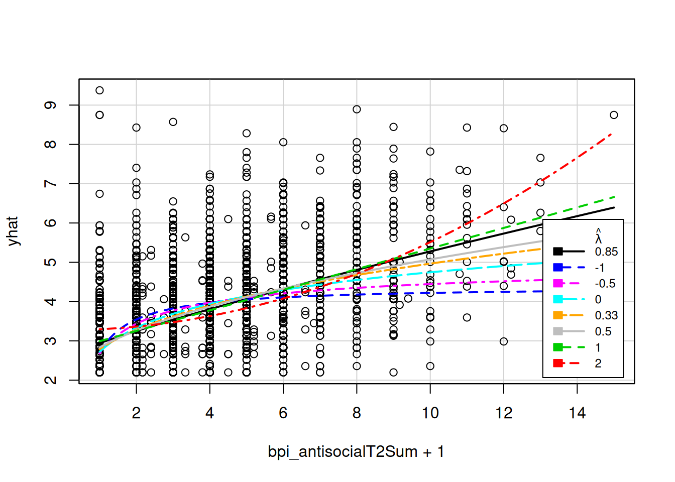
powerTransform(strictlyPositiveDV) Estimated transformation parameter
Y1
0.234032 transformedDV <- powerTransform(strictlyPositiveDV)
summary(transformedDV)bcPower Transformation to Normality
Est Power Rounded Pwr Wald Lwr Bnd Wald Upr Bnd
Y1 0.234 0.23 0.1825 0.2856
Likelihood ratio test that transformation parameter is equal to 0
(log transformation)
LRT df pval
LR test, lambda = (0) 78.04052 1 < 2.22e-16
Likelihood ratio test that no transformation is needed
LRT df pval
LR test, lambda = (1) 853.8675 1 < 2.22e-16Transform the DV
Compare residuals from model with and without transformation
Model without transformation
Call:
lm(formula = bpi_antisocialT2Sum + 1 ~ bpi_antisocialT1Sum +
    bpi_anxiousDepressedSum, data = mydata, na.action = na.exclude)

Residuals:
    Min      1Q  Median      3Q     Max
-8.3755 -1.2337 -0.2212  0.9911 12.8017

Coefficients:
                        Estimate Std. Error t value Pr(>|t|)
(Intercept)              2.19830    0.05983  36.743  < 2e-16 ***
bpi_antisocialT1Sum      0.46553    0.01858  25.049  < 2e-16 ***
bpi_anxiousDepressedSum  0.16075    0.02916   5.513 3.83e-08 ***
---
Signif. codes:  0 '***' 0.001 '**' 0.01 '*' 0.05 '.' 0.1 ' ' 1

Residual standard error: 1.979 on 2871 degrees of freedom
  (8656 observations deleted due to missingness)
Multiple R-squared:  0.262, Adjusted R-squared:  0.2615
F-statistic: 509.6 on 2 and 2871 DF,  p-value: < 2.2e-16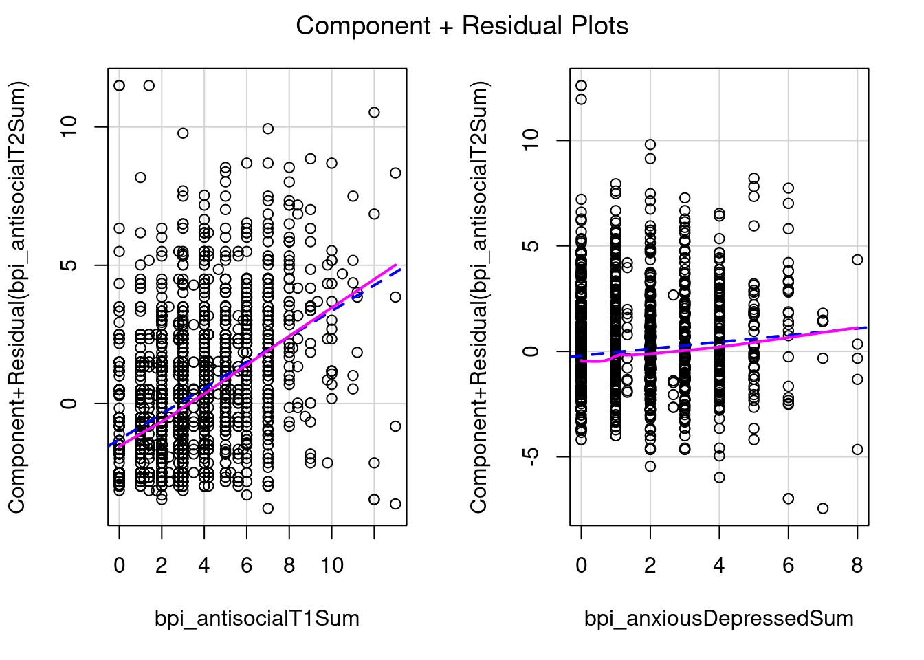
Model with transformation
Call:
lm(formula = bpi_antisocialT2SumTransformed ~ bpi_antisocialT1Sum +
    bpi_anxiousDepressedSum, data = mydata, na.action = na.exclude)

Residuals:
    Min      1Q  Median      3Q     Max
-3.3429 -0.4868  0.0096  0.4922  2.9799

Coefficients:
                        Estimate Std. Error t value Pr(>|t|)
(Intercept)             0.800373   0.022024  36.342  < 2e-16 ***
bpi_antisocialT1Sum     0.165476   0.006841  24.189  < 2e-16 ***
bpi_anxiousDepressedSum 0.055910   0.010733   5.209 2.03e-07 ***
---
Signif. codes:  0 '***' 0.001 '**' 0.01 '*' 0.05 '.' 0.1 ' ' 1

Residual standard error: 0.7283 on 2871 degrees of freedom
  (8656 observations deleted due to missingness)
Multiple R-squared:  0.2477,    Adjusted R-squared:  0.2472
F-statistic: 472.7 on 2 and 2871 DF,  p-value: < 2.2e-16
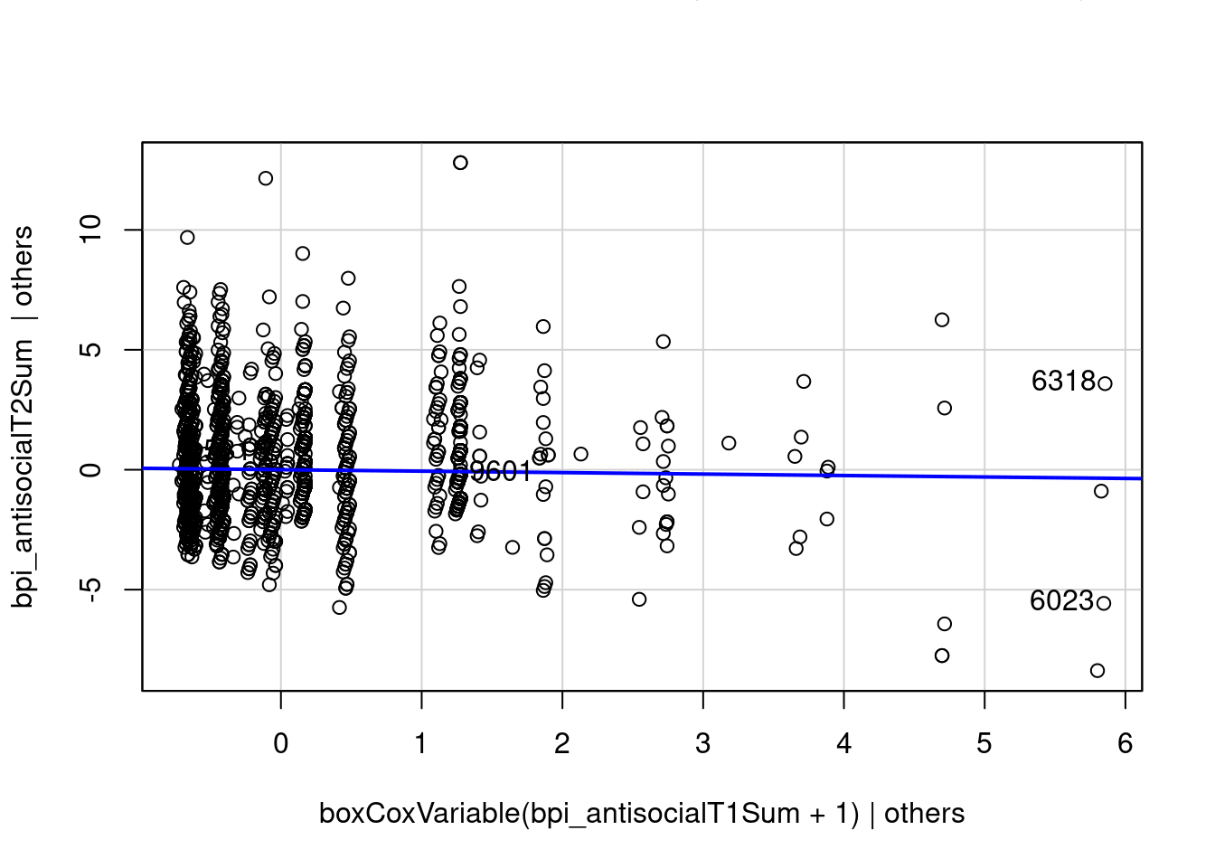
Constructed Variable Test & Plot
A significant p-value indicates a strong need to transform variable:
multipleRegressionModel_constructedVariable <- update(
  multipleRegressionModel,
  . ~ . + boxCoxVariable(bpi_antisocialT1Sum + 1))
summary(multipleRegressionModel_constructedVariable)$coef["boxCoxVariable(bpi_antisocialT1Sum + 1)", , drop = FALSE]
Estimate Std. Error t value
boxCoxVariable(bpi_antisocialT1Sum + 1) -0.06064732 0.04683415 -1.294938
Pr(>|t|)
boxCoxVariable(bpi_antisocialT1Sum + 1) 0.1954457Plot allows us to see whether the need for transformation is spread through data or whether it is just dependent on a small fraction of observations:
avPlots(multipleRegressionModel_constructedVariable, "boxCoxVariable(bpi_antisocialT1Sum + 1)")
Inverse Response Plot
The black line is the best-fitting power transformation:
Useful if the outcome is not strictly positive.
yjPower(DV, lambda)Linear model:
crPlots(multipleRegressionModelNoMissing, order = 1)Error:
! object 'multipleRegressionModelNoMissing' not foundQuadratic model:
crPlots(multipleRegressionModelNoMissing, order = 2)Error:
! object 'multipleRegressionModelNoMissing' not found
Call:
lm(formula = bpi_antisocialT2Sum ~ bpi_antisocialT1Sum + I(bpi_antisocialT1Sum^2) +
    bpi_anxiousDepressedSum, data = mydata, na.action = na.exclude)

Residuals:
    Min      1Q  Median      3Q     Max
-7.6238 -1.2610 -0.2484  0.9923 12.9008

Coefficients:
                          Estimate Std. Error t value Pr(>|t|)
(Intercept)               1.099237   0.076509  14.367  < 2e-16 ***
bpi_antisocialT1Sum       0.547680   0.043723  12.526  < 2e-16 ***
I(bpi_antisocialT1Sum^2) -0.010221   0.004925  -2.075    0.038 *
bpi_anxiousDepressedSum   0.161734   0.029144   5.549 3.13e-08 ***
---
Signif. codes:  0 '***' 0.001 '**' 0.01 '*' 0.05 '.' 0.1 ' ' 1

Residual standard error: 1.977 on 2870 degrees of freedom
  (8656 observations deleted due to missingness)
Multiple R-squared:  0.2631,    Adjusted R-squared:  0.2623
F-statistic: 341.5 on 3 and 2870 DF, p-value: < 2.2e-16anova(
multipleRegressionModel_quadratic,
multipleRegressionModel)crPlots(multipleRegressionModel_quadratic, order = 1)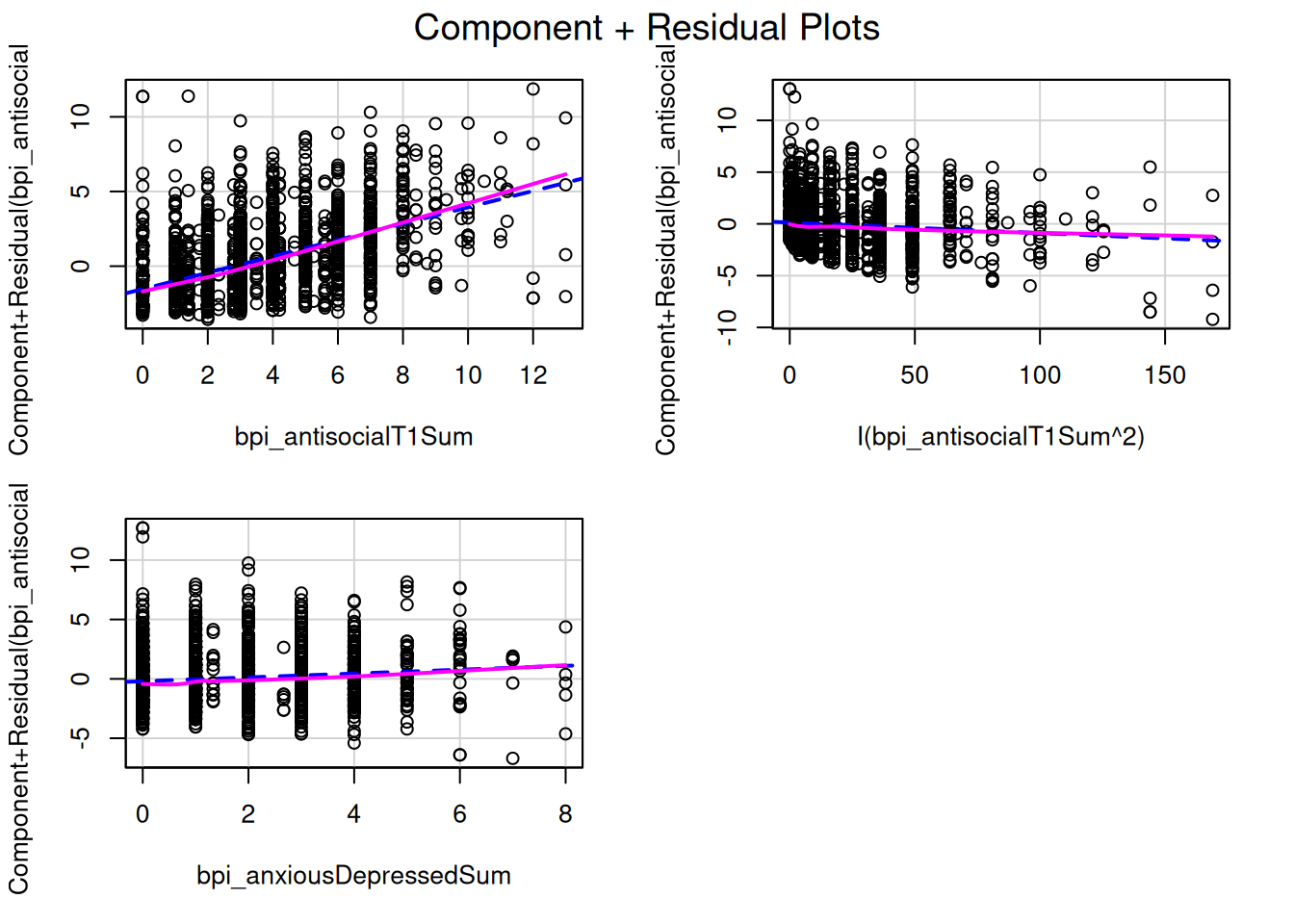
Useful when nonlinear associations among the predictors are very strong (component-plus-residual plots may appear nonlinear even though the true partial regression is linear, a phenonomen called leakage)
ceresPlots(multipleRegressionModel)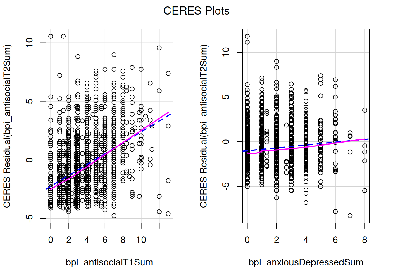
ceresPlots(multipleRegressionModel_quadratic)Error in `plot.window()`:
! need finite 'ylim' values
predictors must be strictly positive (or add a constant to make it strictly positive)
boxTidwell(
  bpi_antisocialT2Sum ~ I(bpi_antisocialT1Sum + 1) + I(bpi_anxiousDepressedSum + 1),
  other.x = NULL, #list variables not to be transformed in other.x
  data = mydata,
  na.action = na.exclude)
MLE of lambda Score Statistic (t) Pr(>|t|)
I(bpi_antisocialT1Sum + 1) 0.90820 -1.0591 0.2897
I(bpi_anxiousDepressedSum + 1) 0.36689 -1.0650 0.2870
iterations = 4
Score test for null hypothesis that all lambdas = 1:
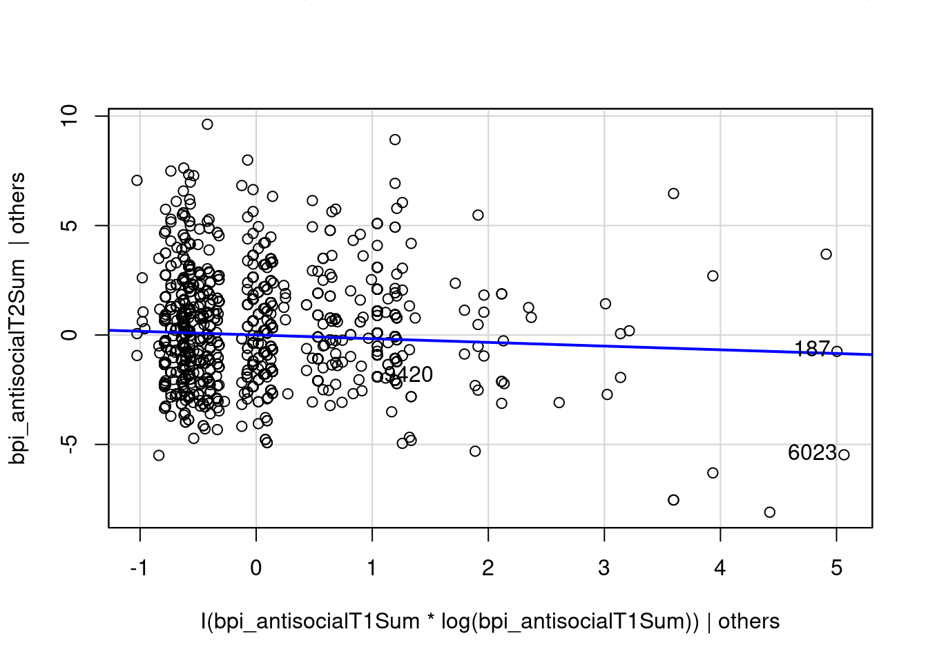
F = 1.4056, df = 2 and 2869, Pr(>F) = 0.2454multipleRegressionModel_cv <- lm(
bpi_antisocialT2Sum ~ I(bpi_antisocialT1Sum + 1) + I(bpi_anxiousDepressedSum + 1) + I(bpi_antisocialT1Sum * log(bpi_antisocialT1Sum)) + I(bpi_anxiousDepressedSum * log(bpi_anxiousDepressedSum)),
data = mydata,
na.action = na.exclude)
summary(multipleRegressionModel_cv)$coef["I(bpi_antisocialT1Sum * log(bpi_antisocialT1Sum))", , drop = FALSE] Estimate Std. Error
I(bpi_antisocialT1Sum * log(bpi_antisocialT1Sum)) -0.1691003 0.06887107
t value Pr(>|t|)
I(bpi_antisocialT1Sum * log(bpi_antisocialT1Sum)) -2.455317 0.01418393summary(multipleRegressionModel_cv)$coef["I(bpi_anxiousDepressedSum * log(bpi_anxiousDepressedSum))", , drop = FALSE] Estimate Std. Error
I(bpi_anxiousDepressedSum * log(bpi_anxiousDepressedSum)) 0.00828867 0.1384918
t value Pr(>|t|)
I(bpi_anxiousDepressedSum * log(bpi_anxiousDepressedSum)) 0.05984953 0.9522831avPlots(multipleRegressionModel_cv, "I(bpi_antisocialT1Sum * log(bpi_antisocialT1Sum))")
avPlots(multipleRegressionModel_cv, "I(bpi_anxiousDepressedSum * log(bpi_anxiousDepressedSum))")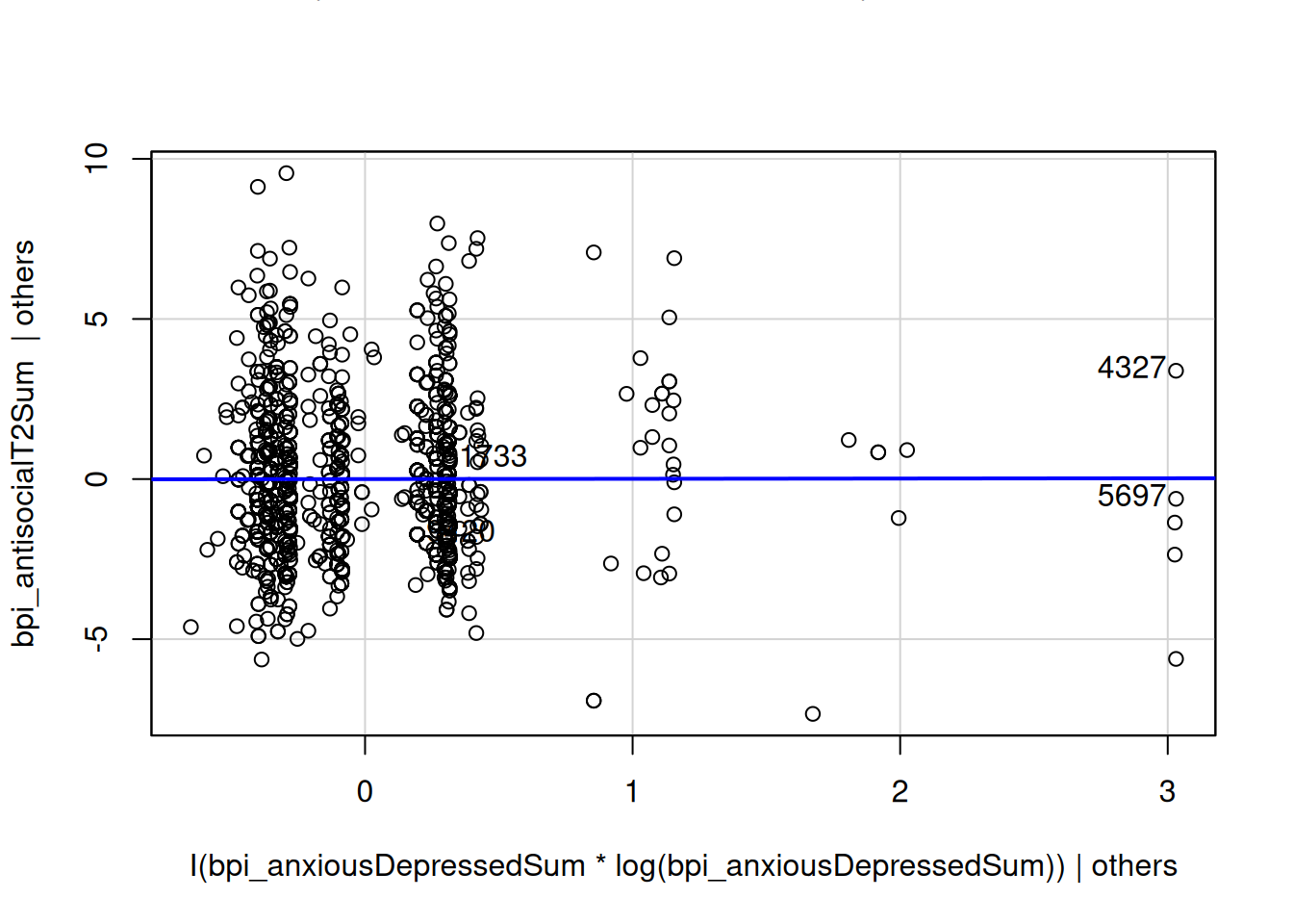
Resources
Spearman’s rho
Spearman’s rho is a non-parametric correlation.
cor.test(
  mydata$bpi_antisocialT1Sum,
  mydata$bpi_antisocialT2Sum) #Pearson r, correlation that is sensitive to outliers
    Pearson's product-moment correlation

data:  mydata$bpi_antisocialT1Sum and mydata$bpi_antisocialT2Sum
t = 31.274, df = 2873, p-value < 2.2e-16
alternative hypothesis: true correlation is not equal to 0
95 percent confidence interval:
 0.4761758 0.5307381
sample estimates:
      cor
0.5039595 cor.test(
mydata$bpi_antisocialT1Sum,
mydata$bpi_antisocialT2Sum, method = "spearman") #Spearman's rho, a rank correlation that is less sensitive to outliers
    Spearman's rank correlation rho

data:  mydata$bpi_antisocialT1Sum and mydata$bpi_antisocialT2Sum
S = 1997347186, p-value < 2.2e-16
alternative hypothesis: true rho is not equal to 0
sample estimates:
      rho
0.4956973
Minimum vollume ellipsoid
$center
bpi_antisocialT1Sum bpi_antisocialT2Sum
           2.056773            1.952882

$cov
                    bpi_antisocialT1Sum bpi_antisocialT2Sum
bpi_antisocialT1Sum           2.1044887           0.8162201
bpi_antisocialT2Sum           0.8162201           2.1211668

$msg
[1] "159 singular samples of size 3 out of 1500"

$crit
[1] 3.79572

$best
[1]  1  3  8  9 10 12

$cor
                    bpi_antisocialT1Sum bpi_antisocialT2Sum
bpi_antisocialT1Sum           1.0000000           0.3863195
bpi_antisocialT2Sum           0.3863195           1.0000000

$n.obs
[1] 2875
Minimum covariance determinant
$center
bpi_antisocialT1Sum bpi_antisocialT2Sum
           2.181181            2.094954

$cov
                    bpi_antisocialT1Sum bpi_antisocialT2Sum
bpi_antisocialT1Sum            2.379036            1.096437
bpi_antisocialT2Sum            1.096437            2.482409

$msg
[1] "154 singular samples of size 3 out of 1500"

$crit
[1] -0.3839279

$best
[1]  1  3  8  9 10 12

$cor
                    bpi_antisocialT1Sum bpi_antisocialT2Sum
bpi_antisocialT1Sum           1.0000000           0.4511764
bpi_antisocialT2Sum           0.4511764           1.0000000

$n.obs
[1] 2875
Winsorized correlation
correlation(
  mydata[,c("bpi_antisocialT1Sum","bpi_antisocialT2Sum")],
  winsorize = 0.2,
  p_adjust = "none")
Percentage bend correlation
correlation(
  mydata[,c("bpi_antisocialT1Sum","bpi_antisocialT2Sum")],
  method = "percentage",
  p_adjust = "none")
Biweight midcorrelation
correlation(
  mydata[,c("bpi_antisocialT1Sum","bpi_antisocialT2Sum")],
  method = "biweight",
  p_adjust = "none")
Xi (\(\xi\))
Xi (\(\xi\)) is an index of the degree of dependence between two variables
Chatterjee, S. (2021). A new coefficient of correlation. Journal of the American Statistical Association, 116(536), 2009-2022. https://doi.org/10.1080/01621459.2020.1758115
Theil-Sen estimator
The Theil-Sen single median estimator is robust to outliers; have to remove missing values first
Call:
mblm(formula = bpi_antisocialT2Sum ~ bpi_antisocialT1Sum, dataframe = mydata_subset,
    repeated = FALSE)

Coefficients:
        (Intercept)  bpi_antisocialT1Sum
1.0 0.6 Best when no outliers: MM-type regression estimator
Robust linear regression
MM-type regression estimator (best):
lmrob(
  bpi_antisocialT2Sum ~ bpi_antisocialT1Sum + bpi_anxiousDepressedSum,
  data = mydata,
  na.action = na.exclude)
Call:
lmrob(formula = bpi_antisocialT2Sum ~ bpi_antisocialT1Sum + bpi_anxiousDepressedSum,     data = mydata, na.action = na.exclude)
 \--> method = "MM"
Coefficients:
            (Intercept)      bpi_antisocialT1Sum  bpi_anxiousDepressedSum
                 0.9440                   0.4914                   0.1577
Iteratively reweighted least squares (IRLS): http://www.ats.ucla.edu/stat/r/dae/rreg.htm (archived at https://web.archive.org/web/20161119025907/http://www.ats.ucla.edu/stat/r/dae/rreg.htm)
rlm(
  bpi_antisocialT2Sum ~ bpi_antisocialT1Sum + bpi_anxiousDepressedSum,
  data = mydata,
  na.action = na.exclude)
Call:
rlm(formula = bpi_antisocialT2Sum ~ bpi_antisocialT1Sum + bpi_anxiousDepressedSum,
data = mydata, na.action = na.exclude)
Converged in 6 iterations
Coefficients:
(Intercept) bpi_antisocialT1Sum bpi_anxiousDepressedSum
0.9838033 0.4873118 0.1620020
Degrees of freedom: 2874 total; 2871 residual
(8656 observations deleted due to missingness)
Scale estimate: 1.62 Robust generalized regression
glmrob(
  bpi_antisocialT2Sum ~ bpi_antisocialT1Sum + bpi_anxiousDepressedSum,
  data = mydata,
  family = "poisson",
  na.action = "na.exclude")
Call:  glmrob(formula = bpi_antisocialT2Sum ~ bpi_antisocialT1Sum +      bpi_anxiousDepressedSum, family = "poisson", data = mydata,      na.action = "na.exclude")

Coefficients:
            (Intercept)      bpi_antisocialT1Sum  bpi_anxiousDepressedSum
                0.37281                  0.15589                  0.05026

Number of observations: 2874
Fitted by method  'Mqle'
Most resistant to outliers: Least trimmed squares (LTS)—but not good as a standalone estimator, better for identifying outliers
ltsReg(
  bpi_antisocialT2Sum ~ bpi_antisocialT1Sum + bpi_anxiousDepressedSum,
  data = mydata,
  na.action = na.exclude)
Call:
ltsReg.formula(formula = bpi_antisocialT2Sum ~ bpi_antisocialT1Sum +     bpi_anxiousDepressedSum, data = mydata, na.action = na.exclude)

Coefficients:
              Intercept      bpi_antisocialT1Sum  bpi_anxiousDepressedSum
                 0.7813                   0.5145                   0.1318

Scale estimate 1.75
Not great options:
Quantile (L1) regression: rq() function of quantreg package
https://data.library.virginia.edu/getting-started-with-quantile-regression/ (archived at https://perma.cc/FSV4-5DCR)
quantiles <- 1:9/10

quantileRegressionModel <- rq(
  bpi_antisocialT2Sum ~ bpi_antisocialT1Sum + bpi_anxiousDepressedSum,
  data = mydata,
  tau = quantiles,
  na.action = na.exclude)

quantileRegressionModel
Call:
rq(formula = bpi_antisocialT2Sum ~ bpi_antisocialT1Sum + bpi_anxiousDepressedSum,
tau = quantiles, data = mydata, na.action = na.exclude)
Coefficients:
tau= 0.1 tau= 0.2 tau= 0.3 tau= 0.4 tau= 0.5
(Intercept) -0.19607843 0.0000000 0.09090909 0.5 0.88
bpi_antisocialT1Sum 0.19607843 0.3333333 0.45454545 0.5 0.52
bpi_anxiousDepressedSum 0.09803922 0.1111111 0.13636364 0.1 0.12
tau= 0.6 tau= 0.7 tau= 0.8 tau= 0.9
(Intercept) 1.0000000 1.3750 2.1250 3.1000000
bpi_antisocialT1Sum 0.5913978 0.6250 0.6250 0.6428571
bpi_anxiousDepressedSum 0.2043011 0.1875 0.1875 0.2285714
Degrees of freedom: 11530 total; 11527 residualsummary(quantileRegressionModel)
Call: rq(formula = bpi_antisocialT2Sum ~ bpi_antisocialT1Sum + bpi_anxiousDepressedSum,
    tau = quantiles, data = mydata, na.action = na.exclude)

tau: [1] 0.1

Coefficients:
                        Value    Std. Error t value  Pr(>|t|)
(Intercept)             -0.19608  0.05341   -3.67101  0.00025
bpi_antisocialT1Sum      0.19608  0.03492    5.61452  0.00000
bpi_anxiousDepressedSum  0.09804  0.03536    2.77276  0.00559

Call: rq(formula = bpi_antisocialT2Sum ~ bpi_antisocialT1Sum + bpi_anxiousDepressedSum,
    tau = quantiles, data = mydata, na.action = na.exclude)

tau: [1] 0.2

Coefficients:
                        Value    Std. Error t value  Pr(>|t|)
(Intercept)              0.00000  0.04196    0.00000  1.00000
bpi_antisocialT1Sum      0.33333  0.02103   15.85299  0.00000
bpi_anxiousDepressedSum  0.11111  0.02669    4.16376  0.00003

Call: rq(formula = bpi_antisocialT2Sum ~ bpi_antisocialT1Sum + bpi_anxiousDepressedSum,
    tau = quantiles, data = mydata, na.action = na.exclude)

tau: [1] 0.3

Coefficients:
                        Value    Std. Error t value  Pr(>|t|)
(Intercept)              0.09091  0.05830    1.55945  0.11900
bpi_antisocialT1Sum      0.45455  0.02584   17.59380  0.00000
bpi_anxiousDepressedSum  0.13636  0.03601    3.78723  0.00016

Call: rq(formula = bpi_antisocialT2Sum ~ bpi_antisocialT1Sum + bpi_anxiousDepressedSum,
    tau = quantiles, data = mydata, na.action = na.exclude)

tau: [1] 0.4

Coefficients:
                        Value    Std. Error t value  Pr(>|t|)
(Intercept)              0.50000  0.06410    7.80035  0.00000
bpi_antisocialT1Sum      0.50000  0.02374   21.06425  0.00000
bpi_anxiousDepressedSum  0.10000  0.03372    2.96584  0.00304

Call: rq(formula = bpi_antisocialT2Sum ~ bpi_antisocialT1Sum + bpi_anxiousDepressedSum,
    tau = quantiles, data = mydata, na.action = na.exclude)

tau: [1] 0.5

Coefficients:
                        Value    Std. Error t value  Pr(>|t|)
(Intercept)              0.88000  0.06584   13.36547  0.00000
bpi_antisocialT1Sum      0.52000  0.02491   20.87561  0.00000
bpi_anxiousDepressedSum  0.12000  0.03771    3.18245  0.00148

Call: rq(formula = bpi_antisocialT2Sum ~ bpi_antisocialT1Sum + bpi_anxiousDepressedSum,
    tau = quantiles, data = mydata, na.action = na.exclude)

tau: [1] 0.6

Coefficients:
                        Value    Std. Error t value  Pr(>|t|)
(Intercept)              1.00000  0.04246   23.55356  0.00000
bpi_antisocialT1Sum      0.59140  0.02146   27.55553  0.00000
bpi_anxiousDepressedSum  0.20430  0.03156    6.47422  0.00000

Call: rq(formula = bpi_antisocialT2Sum ~ bpi_antisocialT1Sum + bpi_anxiousDepressedSum,
    tau = quantiles, data = mydata, na.action = na.exclude)

tau: [1] 0.7

Coefficients:
                        Value    Std. Error t value  Pr(>|t|)
(Intercept)              1.37500  0.07716   17.82011  0.00000
bpi_antisocialT1Sum      0.62500  0.02397   26.07659  0.00000
bpi_anxiousDepressedSum  0.18750  0.03760    4.98623  0.00000

Call: rq(formula = bpi_antisocialT2Sum ~ bpi_antisocialT1Sum + bpi_anxiousDepressedSum,
    tau = quantiles, data = mydata, na.action = na.exclude)

tau: [1] 0.8

Coefficients:
                        Value    Std. Error t value  Pr(>|t|)
(Intercept)              2.12500  0.09498   22.37224  0.00000
bpi_antisocialT1Sum      0.62500  0.03524   17.73509  0.00000
bpi_anxiousDepressedSum  0.18750  0.05040    3.72020  0.00020

Call: rq(formula = bpi_antisocialT2Sum ~ bpi_antisocialT1Sum + bpi_anxiousDepressedSum,
    tau = quantiles, data = mydata, na.action = na.exclude)

tau: [1] 0.9

Coefficients:
                        Value    Std. Error t value  Pr(>|t|)
(Intercept)              3.10000  0.11730   26.42749  0.00000
bpi_antisocialT1Sum      0.64286  0.04797   13.40136  0.00000
bpi_anxiousDepressedSum  0.22857  0.06439    3.54960  0.00039
Plot to examine the association between the predictor and the outcome at different levels (i.e., quantiles) of the predictor:
ggplot(
  mydata,
  aes(bpi_antisocialT1Sum, bpi_antisocialT2Sum)) +
  geom_point() +
  geom_quantile(
    quantiles = quantiles,
    aes(color = factor(after_stat(quantile))))
Below is a plot that examines the difference in quantile coefficients (and associated confidence intervals) at different levels (i.e., quantiles) of the predictor. The x-axis is the quantile of the predictor. The y-axis is the slope coefficient. Each black dot is the slope coefficient for the given quantile of the predictor. The red lines are the least squares estimate of the slope coefficient and its confidence interval.
https://www.ucd.ie/ecomodel/Resources/QQplots_WebVersion.html (archived at https://perma.cc/9UC3-3WRX)
qqPlot(multipleRegressionModel, main = "QQ Plot", id = TRUE)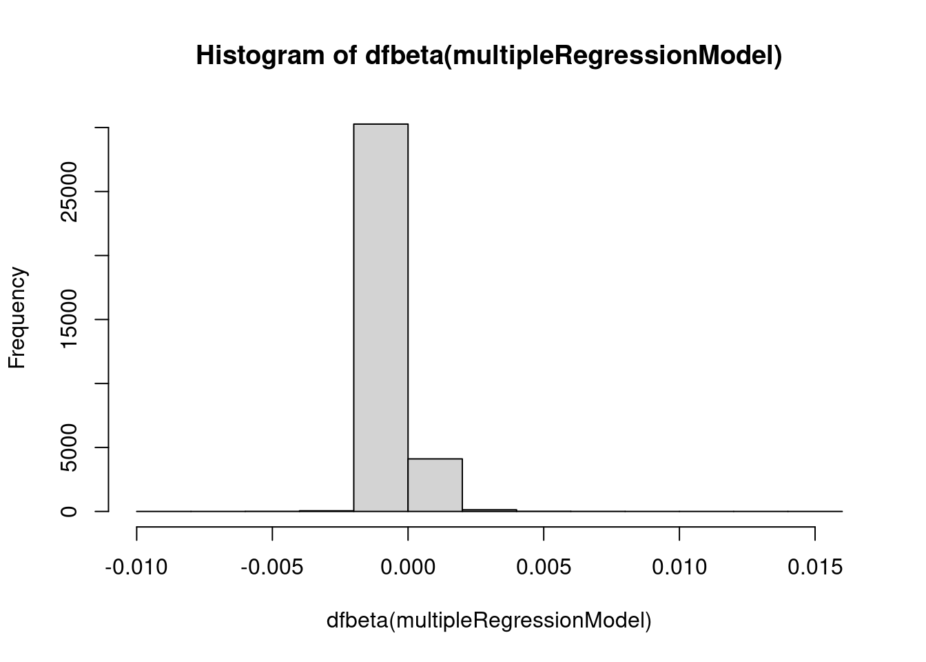
[1] 8955 8956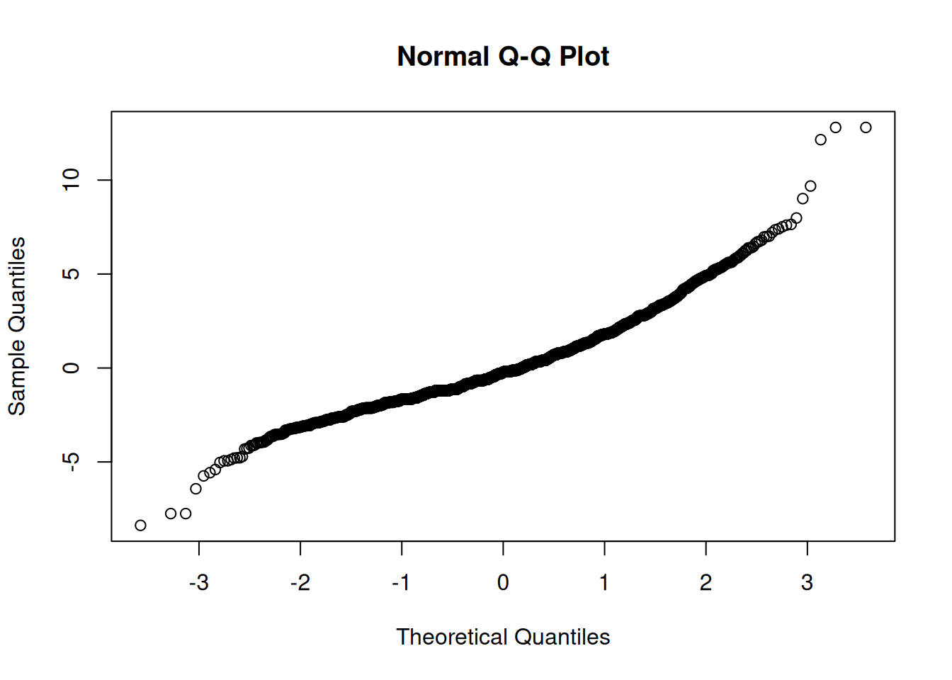

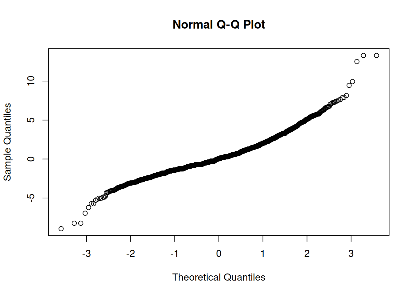
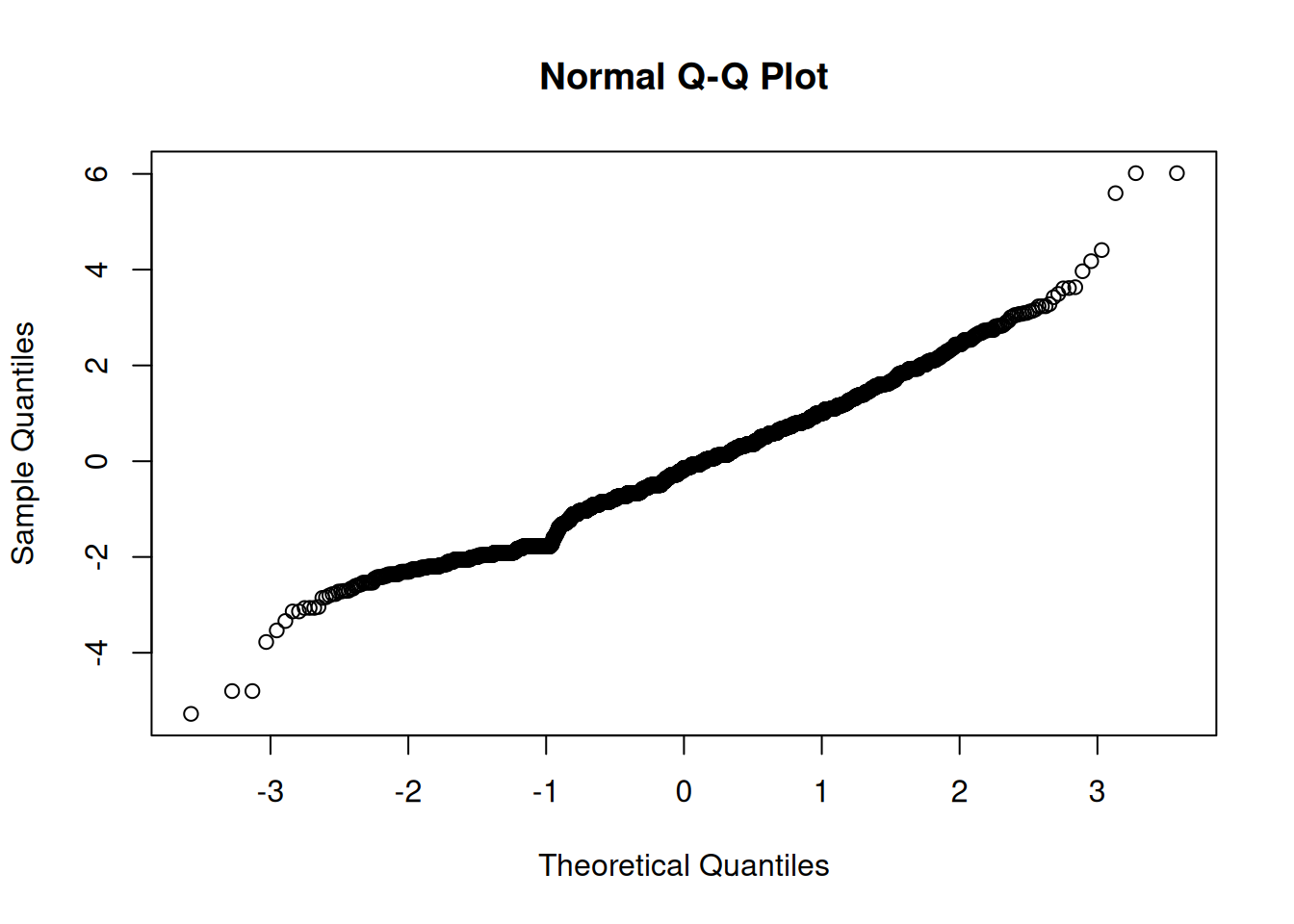
Error in `residuals.Glm()`:
! argument "type" is missing, with no default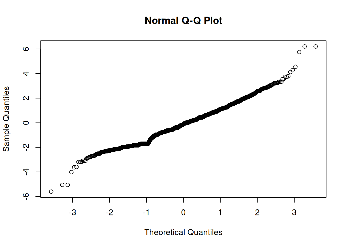
Error in `h()`:
! error in evaluating the argument 'object' in selecting a method for function 'resid': object 'multilevelRegressionModel' not foundResidual plots are plots of the residuals versus observed/fitted values.
Includes plots of a) model residuals versus observed values on predictors and b) model residuals versus model fitted values.
Note: have to remove na.action = na.exclude
Tests include:
residualPlots(
multipleRegressionModelNoMissing,
id = TRUE)Error:
! object 'multipleRegressionModelNoMissing' not foundMarginal model plots are plots of the outcome versus predictors/fitted values.
Includes plots of a) observed outcome values versus values on predictors (ignoring the other predictors) and b) observed outcome values versus model fitted values.
marginalModelPlots(
multipleRegressionModel,
sd = TRUE,
id = TRUE)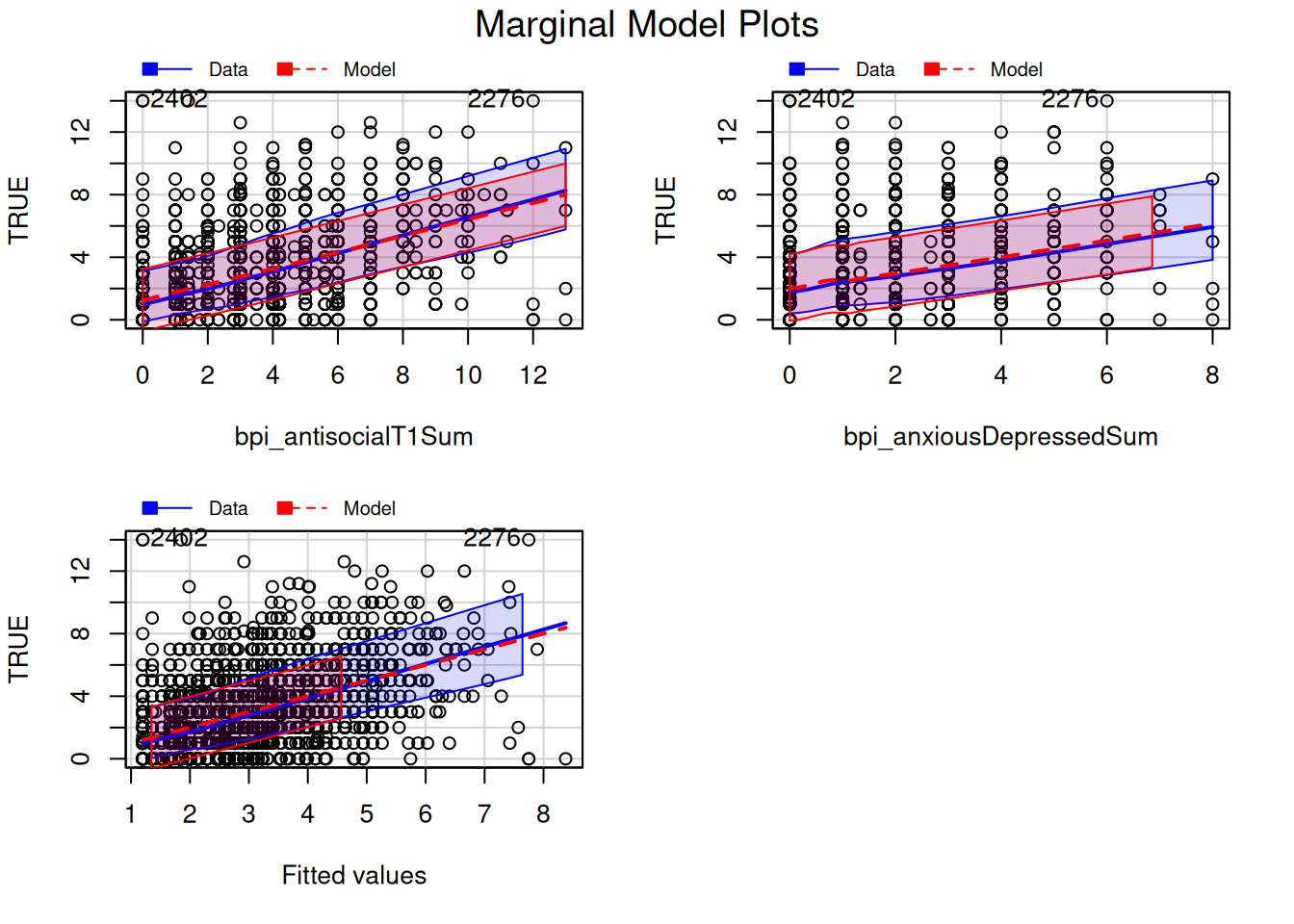
Added-variable plots are plots of the partial association between the outcome and each predictor, controlling for all other predictors.
Useful for identifying jointly influential observations and studying the impact of observations on the regression coefficients.
y-axis: residuals from model with all predictors excluding the predictor of interest
x-axis: residuals from model regressing predictor of interest on all other predictors
avPlots(
multipleRegressionModel,
id = TRUE)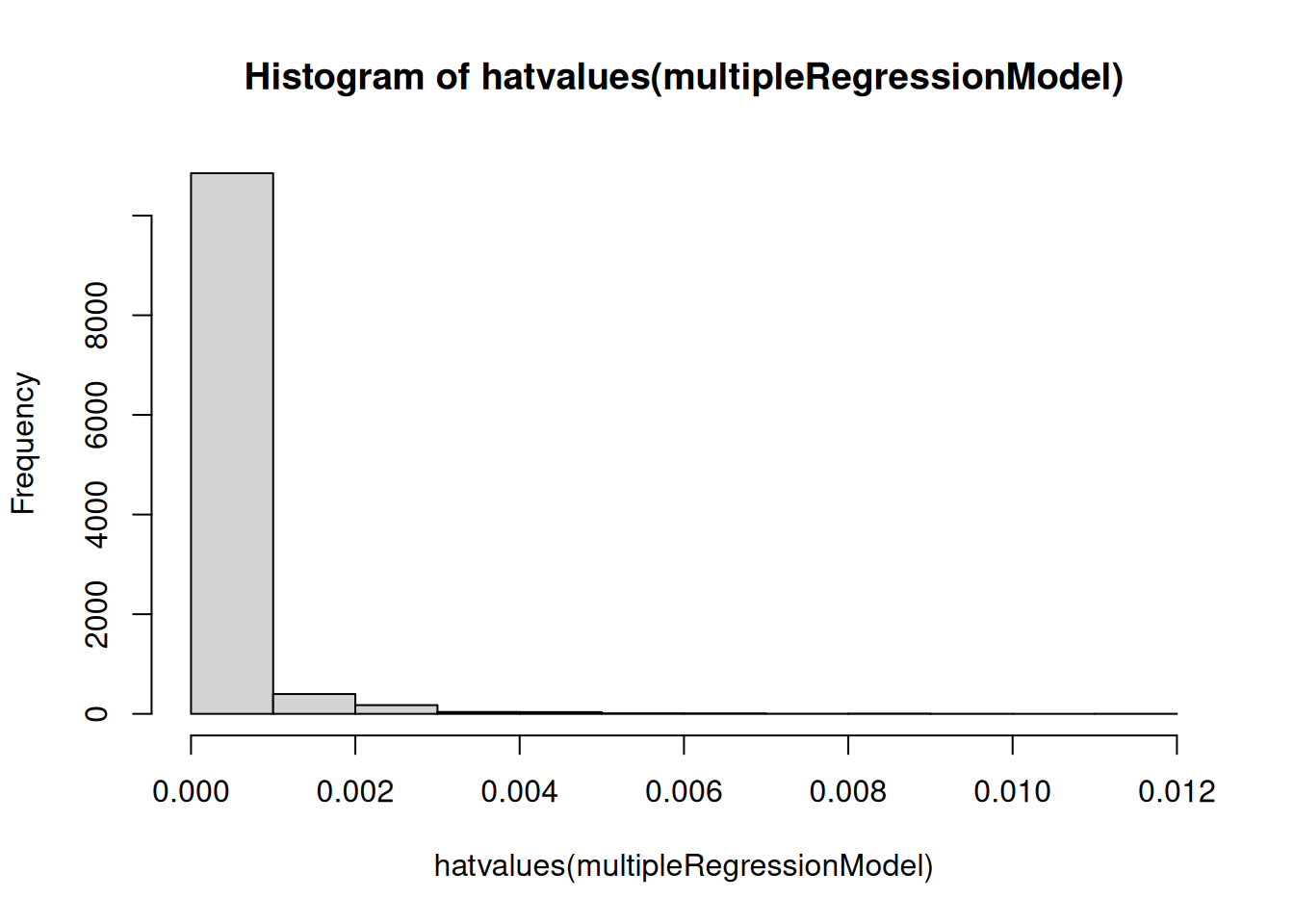
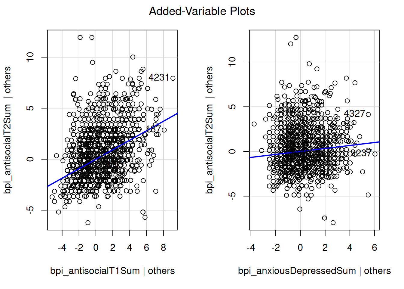
compareCoefs(
multipleRegressionModel,
multipleRegressionModel_removeJointlyInfluentialObs)Calls:
1: lm(formula = bpi_antisocialT2Sum ~ bpi_antisocialT1Sum +
bpi_anxiousDepressedSum, data = mydata, na.action = na.exclude)
2: lm(formula = bpi_antisocialT2Sum ~ bpi_antisocialT1Sum +
bpi_anxiousDepressedSum, data = mydata, subset = -c(6318, 6023, 4022, 4040),
na.action = na.exclude)
Model 1 Model 2
(Intercept) 1.1983 1.1949
SE 0.0598 0.0599
bpi_antisocialT1Sum 0.4655 0.4649
SE 0.0186 0.0188
bpi_anxiousDepressedSum 0.1608 0.1665
SE 0.0292 0.0295
Locates the largest Studentized residuals in absolute value and computes the Bonferroni-corrected p-values based on a t-test for linear models.
Test of outlyingness, i.e., how likely one would have a residual of a given magnitude in a normal distribution with the same sample size
Note: it does not test how extreme an observation is relative to its distribution (i.e., leverage)
outlierTest(multipleRegressionModel) rstudent unadjusted p-value Bonferroni p
8955 6.519574 8.2999e-11 2.3854e-07
8956 6.519574 8.2999e-11 2.3854e-07
8957 6.182195 7.2185e-10 2.0746e-06
2560 4.914941 9.3800e-07 2.6958e-03
1385 4.573975 4.9884e-06 1.4337e-02Identifies observations with high leverage (i.e., high hat values)
hat values are an index of leverage (observations that are far from the center of the regressor space and have greater influence on OLS regression coefficients)


influenceIndexPlot(
multipleRegressionModel,
id = TRUE)
influencePlot(
multipleRegressionModel,
id = TRUE) # circle size is proportional to Cook's Distance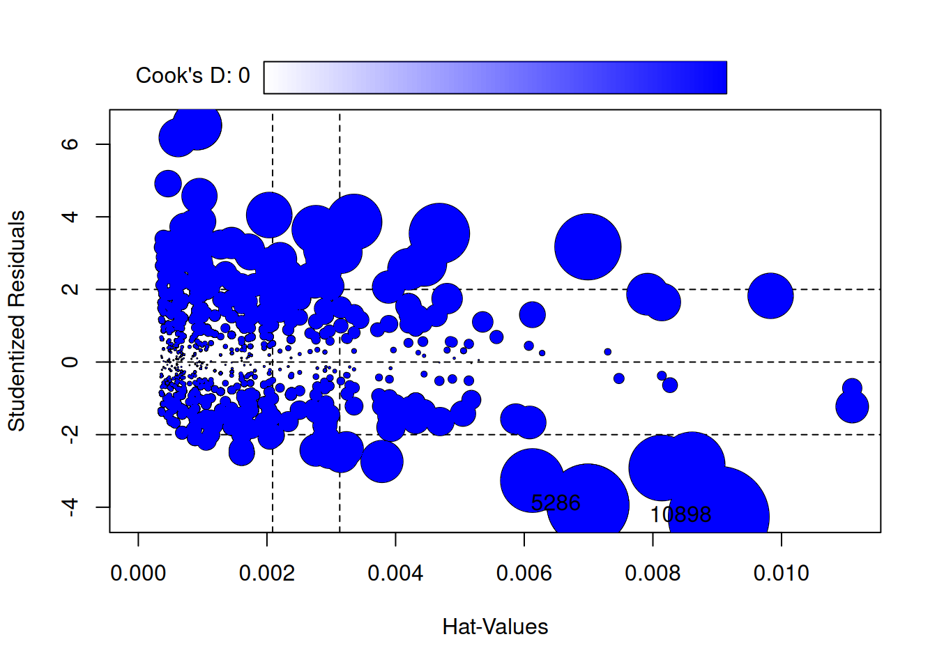
leveragePlots(
multipleRegressionModel,
id = TRUE)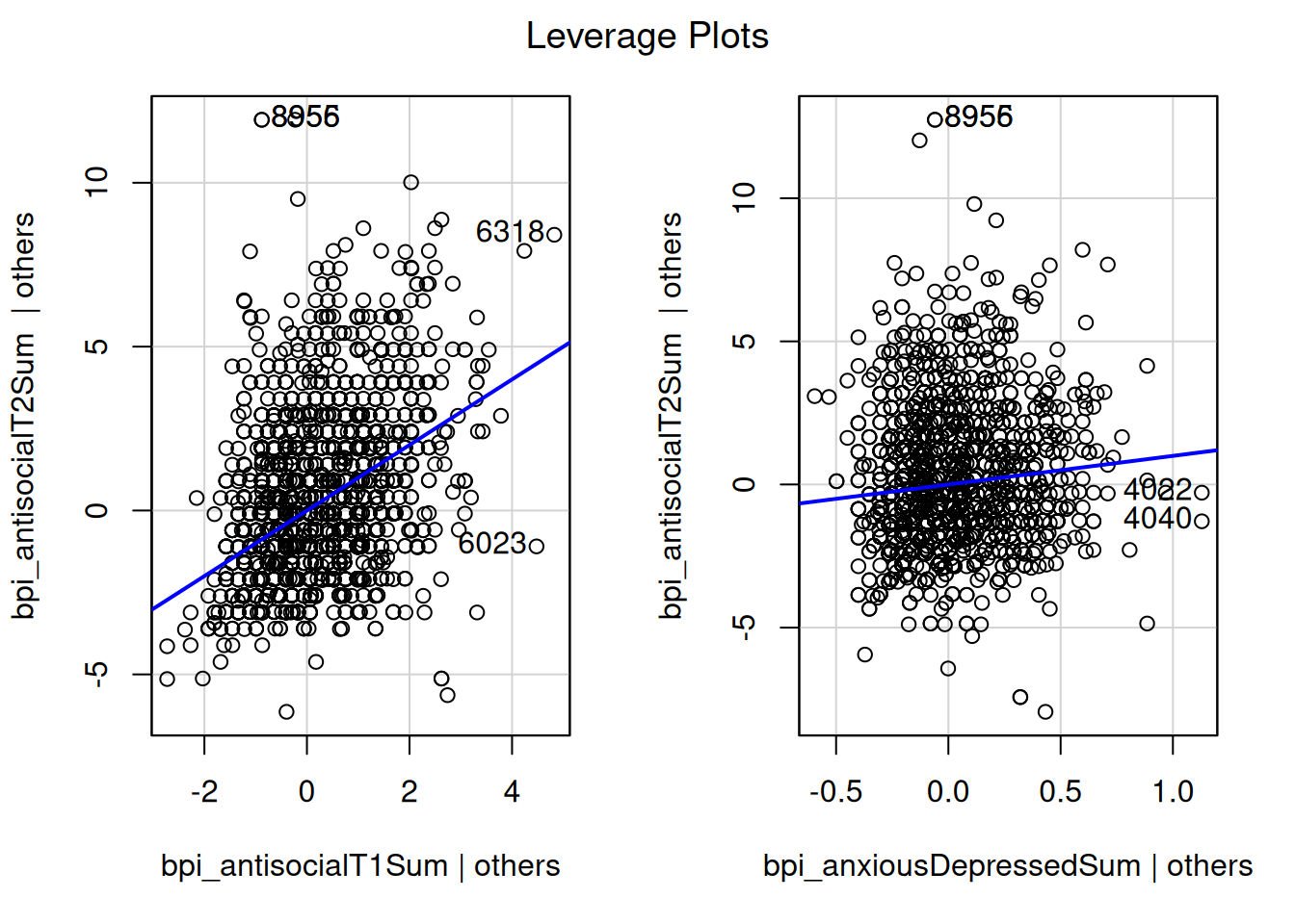
https://cran.r-project.org/web/packages/olsrr/vignettes/influence_measures.html (archived at https://perma.cc/T2TS-PZZ4)
head(influence.measures(multipleRegressionModel)$infmat) dfb.1_ dfb.b_T1 dfb.b_DS dffit cov.r cook.d
1 0.000000000 0.000000000 0.000000000 NA 1.0000000 NA
2 0.000000000 0.000000000 0.000000000 NA 1.0000000 NA
3 -0.006546394 0.008357248 -0.006308529 -0.01004886 1.0024362 0.0000336708
4 0.042862749 -0.025185789 -0.007782877 0.04286275 0.9998621 0.0006121902
5 0.000000000 0.000000000 0.000000000 NA 1.0000000 NA
6 -0.018327367 0.010769006 0.003327823 -0.01832737 1.0015775 0.0001119888
hat
1 0.0000000000
2 0.0000000000
3 0.0014593072
4 0.0009143185
5 0.0000000000
6 0.0009143185 (Intercept) bpi_antisocialT1Sum bpi_anxiousDepressedSum
1 0.0000000000 0.0000000000 0.000000e+00
2 0.0000000000 0.0000000000 0.000000e+00
3 -0.0003917284 0.0001553400 -1.839704e-04
4 0.0025639901 -0.0004679817 -2.268890e-04
5 0.0000000000 0.0000000000 0.000000e+00
6 -0.0010966309 0.0002001580 9.704151e-05
dfbetasPlots(
multipleRegressionModel,
id = TRUE)Error in `dfbetasPlots.lm()`:
! argument 2 matches multiple formal arguments 8472 4468 1917 8955 8956 1986
0.2664075 0.2428065 0.2237760 0.1972271 0.1972271 0.1923034 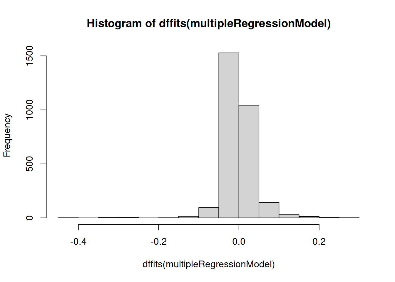
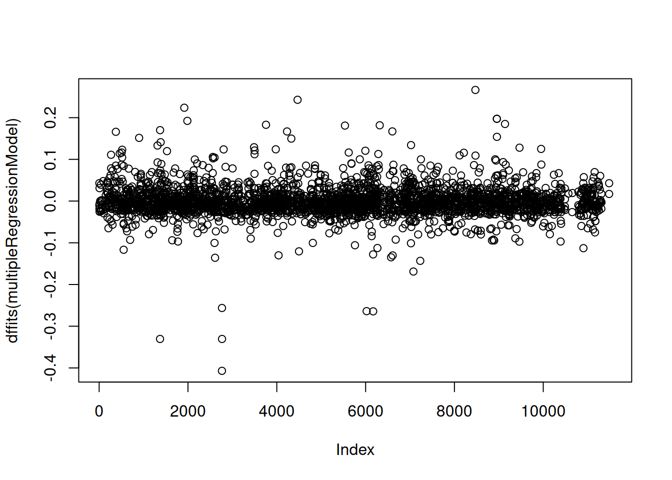

Observations that are both outlying (have a high residual from the regression line) and have high leverage (are far from the center of the regressor space) have high influence on the OLS regression coefficients. An observation will have less influence if it lies on the regression line (not an outlier, i.e., has a low residual) or if it has low leverage (i.e., has a value near the center of a predictor’s distribution).
head(cooks.distance(multipleRegressionModel)[order(cooks.distance(multipleRegressionModel), decreasing = TRUE)]) 2765 1371 2767 8472 6170 6023
0.05488391 0.03624388 0.03624388 0.02358305 0.02323282 0.02315496 hist(cooks.distance(multipleRegressionModel))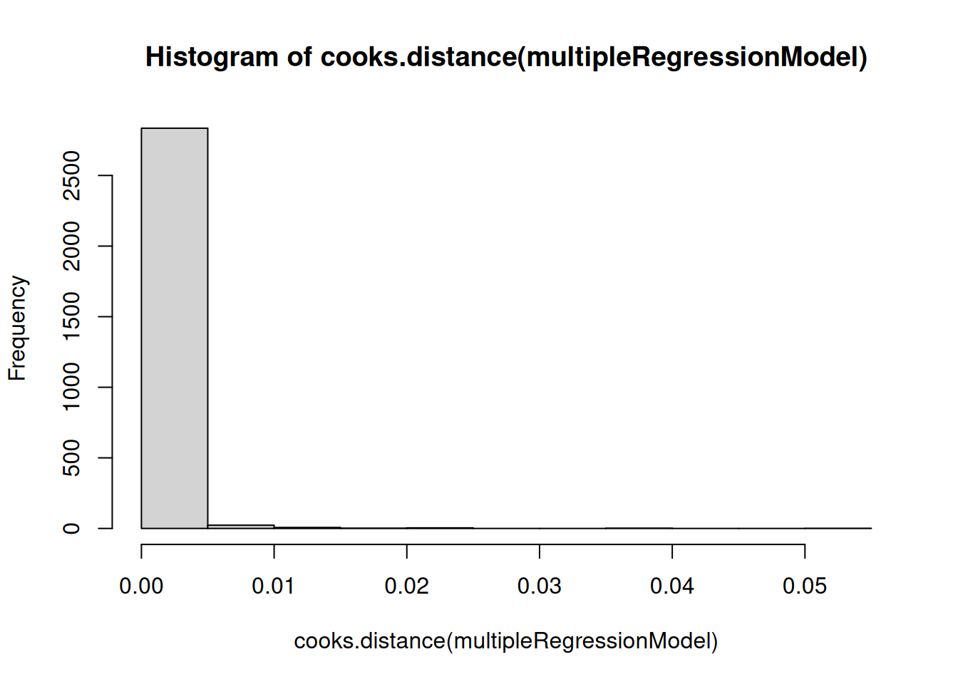
plot(cooks.distance(multipleRegressionModel))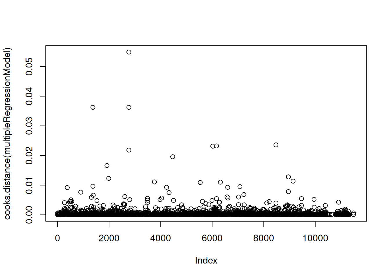
plot(cooks.distance(multipleRegressionModel)[order(cooks.distance(multipleRegressionModel), decreasing = TRUE)])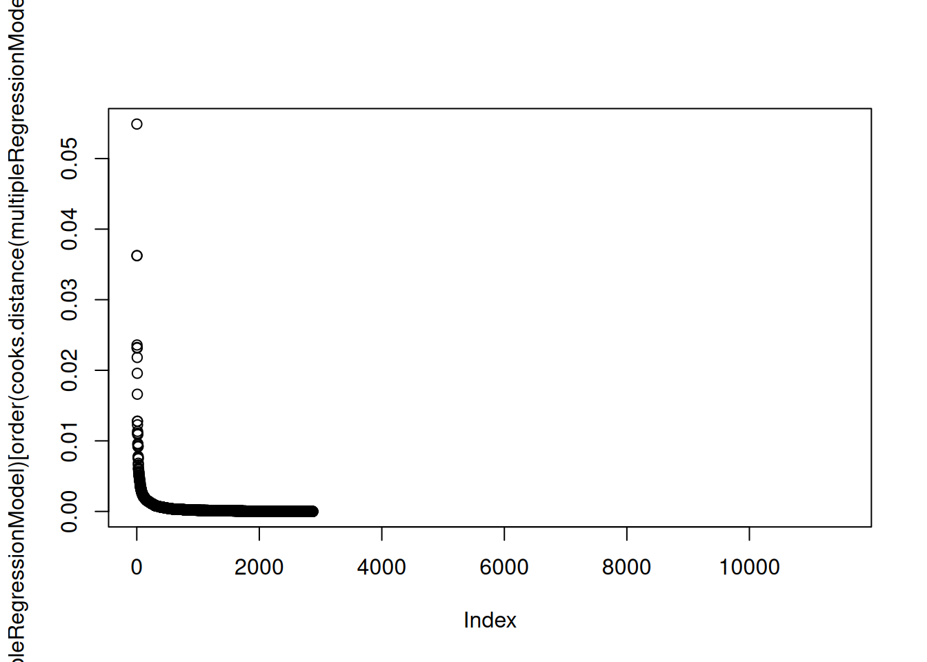
multipleRegressionModel_2 <- lm(
bpi_antisocialT2Sum ~ bpi_antisocialT1Sum + bpi_anxiousDepressedSum,
data = mydata,
na.action = na.exclude,
subset = -c(2765,1371))
multipleRegressionModel_3 <- lm(
bpi_antisocialT2Sum ~ bpi_antisocialT1Sum + bpi_anxiousDepressedSum,
data = mydata,
na.action = na.exclude,
subset = -c(2765,1371,2767))
multipleRegressionModel_4 <- lm(
bpi_antisocialT2Sum ~ bpi_antisocialT1Sum + bpi_anxiousDepressedSum,
data = mydata,
na.action = na.exclude,
subset = -c(2765,1371,2767,8472))
multipleRegressionModel_5 <- lm(
bpi_antisocialT2Sum ~ bpi_antisocialT1Sum + bpi_anxiousDepressedSum,
data = mydata,
na.action = na.exclude,
subset = -c(2765,1371,2767,8472,6170))
multipleRegressionModel_6 <- lm(
bpi_antisocialT2Sum ~ bpi_antisocialT1Sum + bpi_anxiousDepressedSum,
data = mydata,
na.action = na.exclude,
subset = -c(2765,1371,2767,8472,6170,6023))
multipleRegressionModel_7 <- lm(
bpi_antisocialT2Sum ~ bpi_antisocialT1Sum + bpi_anxiousDepressedSum,
data = mydata,
na.action = na.exclude,
subset = -c(2765,1371,2767,8472,6170,6023,2766))compareCoefs(
multipleRegressionModel,
multipleRegressionModel_2,
multipleRegressionModel_3,
multipleRegressionModel_4,
multipleRegressionModel_5,
multipleRegressionModel_6,
multipleRegressionModel_7)Calls:
1: lm(formula = bpi_antisocialT2Sum ~ bpi_antisocialT1Sum +
bpi_anxiousDepressedSum, data = mydata, na.action = na.exclude)
2: lm(formula = bpi_antisocialT2Sum ~ bpi_antisocialT1Sum +
bpi_anxiousDepressedSum, data = mydata, subset = -c(2765, 1371), na.action =
na.exclude)
3: lm(formula = bpi_antisocialT2Sum ~ bpi_antisocialT1Sum +
bpi_anxiousDepressedSum, data = mydata, subset = -c(2765, 1371, 2767),
na.action = na.exclude)
4: lm(formula = bpi_antisocialT2Sum ~ bpi_antisocialT1Sum +
bpi_anxiousDepressedSum, data = mydata, subset = -c(2765, 1371, 2767, 8472),
na.action = na.exclude)
5: lm(formula = bpi_antisocialT2Sum ~ bpi_antisocialT1Sum +
bpi_anxiousDepressedSum, data = mydata, subset = -c(2765, 1371, 2767, 8472,
6170), na.action = na.exclude)
6: lm(formula = bpi_antisocialT2Sum ~ bpi_antisocialT1Sum +
bpi_anxiousDepressedSum, data = mydata, subset = -c(2765, 1371, 2767, 8472,
6170, 6023), na.action = na.exclude)
7: lm(formula = bpi_antisocialT2Sum ~ bpi_antisocialT1Sum +
bpi_anxiousDepressedSum, data = mydata, subset = -c(2765, 1371, 2767, 8472,
6170, 6023, 2766), na.action = na.exclude)
Model 1 Model 2 Model 3 Model 4 Model 5 Model 6 Model 7
(Intercept) 1.1983 1.1704 1.1577 1.1676 1.1620 1.1537 1.1439
SE 0.0598 0.0597 0.0596 0.0596 0.0596 0.0595 0.0595
bpi_antisocialT1Sum 0.4655 0.4739 0.4779 0.4748 0.4744 0.4793 0.4836
SE 0.0186 0.0185 0.0185 0.0185 0.0185 0.0185 0.0185
bpi_anxiousDepressedSum 0.1608 0.1691 0.1726 0.1699 0.1770 0.1742 0.1743
SE 0.0292 0.0290 0.0290 0.0289 0.0290 0.0290 0.0289
(Intercept) bpi_antisocialT1Sum bpi_anxiousDepressedSum
1.1983004 0.4655286 0.1607541 Intercept bpi_antisocialT1Sum bpi_anxiousDepressedSum
0.7439567 0.5432644 0.1524929 Book: An R Companion to Applied Regression
https://people.duke.edu/~rnau/testing.htm (archived at https://perma.cc/9CXH-GBSN)
https://www.statmethods.net/stats/rdiagnostics.html (archived at https://perma.cc/7JX8-K6BY)
https://socserv.socsci.mcmaster.ca/jfox/Courses/Brazil-2009/index.html (archived at https://perma.cc/4A2P-9S49)
https://en.wikipedia.org/wiki/Ordinary_least_squares#Assumptions (archived at https://perma.cc/Q4NS-X8TJ)
R version 4.6.1 (2026-06-24)
Platform: x86_64-pc-linux-gnu
Running under: Ubuntu 24.04.4 LTS
Matrix products: default
BLAS: /usr/lib/x86_64-linux-gnu/openblas-pthread/libblas.so.3
LAPACK: /usr/lib/x86_64-linux-gnu/openblas-pthread/libopenblasp-r0.3.26.so; LAPACK version 3.12.0
locale:
[1] LC_CTYPE=C.UTF-8 LC_NUMERIC=C LC_TIME=C.UTF-8
[4] LC_COLLATE=C.UTF-8 LC_MONETARY=C.UTF-8 LC_MESSAGES=C.UTF-8
[7] LC_PAPER=C.UTF-8 LC_NAME=C LC_ADDRESS=C
[10] LC_TELEPHONE=C LC_MEASUREMENT=C.UTF-8 LC_IDENTIFICATION=C
time zone: UTC
tzcode source: system (glibc)
attached base packages:
[1] stats graphics grDevices utils datasets methods base
other attached packages:
[1] yhat_2.0-5 rockchalk_1.8.164 effectsize_1.0.3 cocor_1.1-4
[5] XICOR_0.4.1 mice_3.19.0 regtools_1.7.0 gtools_3.9.5
[9] FNN_1.1.4.1 lavaan_0.7-2 interactions_1.2.0 correlation_0.8.8
[13] effects_4.2-5 mblm_0.12.1 quantreg_6.1 SparseM_1.84-2
[17] olsrr_0.7.0 foreign_0.8-91 AER_1.2-17 survival_3.8-6
[21] sandwich_3.1-2 lmtest_0.9-40 zoo_1.8-15 mgcv_1.9-4
[25] nlme_3.1-169 car_3.1-5 carData_3.0-6 cvTools_0.3.3
[29] lattice_0.22-9 brms_2.23.0 Rcpp_1.1.2 robustbase_0.99-7
[33] rms_8.1-1 Hmisc_5.2-6 psych_2.6.5 lubridate_1.9.5
[37] forcats_1.0.1 stringr_1.6.0 dplyr_1.2.1 purrr_1.2.2
[41] readr_2.2.0 tidyr_1.3.2 tibble_3.3.1 ggplot2_4.0.3
[45] tidyverse_2.0.0 MASS_7.3-65 petersenlab_1.2.3
loaded via a namespace (and not attached):
[1] domir_1.3.0 splines_4.6.1 polspline_1.1.25
[4] datawizard_1.3.1 rpart_4.1.27 lifecycle_1.0.5
[7] Rdpack_2.6.6 StanHeaders_2.32.10 processx_3.9.0
[10] globals_0.19.1 insight_1.5.2 backports_1.5.1
[13] survey_4.5 magrittr_2.0.5 openxlsx_4.2.8.1
[16] rmarkdown_2.31 plotrix_3.8-14 yaml_2.3.12
[19] otel_0.2.0 text2vec_0.6.6 zip_3.0.1
[22] pkgbuild_1.4.8 DBI_1.3.0 minqa_1.2.8
[25] RColorBrewer_1.1-3 multcomp_1.4-31 abind_1.4-8
[28] quadprog_1.5-8 nnet_7.3-20 TH.data_1.1-5
[31] tensorA_0.36.2.1 psychTools_2.6.4 jtools_2.3.1
[34] float_0.3-3 inline_0.3.21 listenv_1.0.0
[37] nortest_1.0-4 performance_0.17.1 MatrixModels_0.5-4
[40] goftest_1.2-3 bridgesampling_1.2-1 parallelly_1.48.0
[43] codetools_0.2-20 tidyselect_1.2.1 shape_1.4.6.1
[46] bayesplot_1.15.0 farver_2.1.2 lme4_2.0-6
[49] broom.mixed_0.2.9.7 matrixStats_1.5.0 stats4_4.6.1
[52] base64enc_0.1-6 jsonlite_2.0.0 rsparse_0.5.3
[55] mitml_0.4-5 Formula_1.2-5 iterators_1.0.14
[58] foreach_1.5.2 tools_4.6.1 miscTools_0.6-30
[61] yacca_1.4-2 glue_1.8.1 mnormt_2.1.2
[64] gridExtra_2.3.1 pan_2.0 xfun_0.60
[67] distributional_0.8.1 rje_1.12.1 loo_2.10.0
[70] withr_3.0.3 fastmap_1.2.0 mitools_2.4
[73] boot_1.3-32 callr_3.8.0 digest_0.6.39
[76] estimability_2.0.0 timechange_0.4.0 R6_2.6.1
[79] colorspace_2.1-3 mix_1.0-13 RhpcBLASctl_0.23-42
[82] generics_0.1.4 data.table_1.18.4 htmlwidgets_1.6.4
[85] parameters_0.29.2 pkgconfig_2.0.3 gtable_0.3.6
[88] S7_0.2.2 furrr_0.4.0 htmltools_0.5.9
[91] scales_1.4.0 posterior_1.7.0 reformulas_0.4.4
[94] lgr_0.5.2 knitr_1.51 rstudioapi_0.19.0
[97] tzdb_0.5.0 reshape2_1.4.5 coda_0.19-4.1
[100] checkmate_2.3.4 nloptr_2.2.1 parallel_4.6.1
[103] mlapi_0.1.1 pillar_1.11.1 grid_4.6.1
[106] vctrs_0.7.3 jomo_2.7-6 xtable_1.8-8
[109] cluster_2.1.8.2 htmlTable_2.5.0 evaluate_1.0.5
[112] pbivnorm_0.6.0 kutils_1.73 mvtnorm_1.4-2
[115] cli_3.6.6 compiler_4.6.1 rlang_1.3.0
[118] crayon_1.5.3 rstantools_2.6.0 labeling_0.4.3
[121] ps_1.9.3 plyr_1.8.9 rstan_2.32.7
[124] stringi_1.8.7 pander_0.6.6 QuickJSR_1.10.0
[127] viridisLite_0.4.3 glmnet_5.0 Brobdingnag_1.2-9
[130] bayestestR_0.18.1 Matrix_1.7-5 hms_1.1.4
[133] future_1.75.0 rbibutils_2.4.1 broom_1.0.13
[136] RcppParallel_5.1.11-2 DEoptimR_1.2-0