Code
#install.packages("remotes")
#remotes::install_github("DevPsyLab/petersenlab")For a resource on using lavaan in R for structural equation modeling, see the following e-book: https://tdjorgensen.github.io/SEM-in-Ed-compendium
#install.packages("remotes")
#remotes::install_github("DevPsyLab/petersenlab")options(scipen = 999)set.seed(52242)
sampleSize <- 100
X <- rnorm(sampleSize)
M <- 0.5*X + rnorm(sampleSize)
Y <- 0.7*M + rnorm(sampleSize)
mydata <- data.frame(
X = X,
Y = Y,
M = M)longitudinalMI <- read.csv("./data/Bliese-Ployhart-2002-indicators-1.csv")lavaan SyntaxAdapted from https://osf.io/2y67f/files/q2prk
=~ creates reflective latent variables (is measured by)
latent =~ variable1 + variable2 …=~ names from the dataset<~ creates formative latent variables (is influenced by)
latent <~ variable1 + variable2<~ names from the dataset~ indicates regression
Y ~ XY is influenced by X (i.e., X predicts Y)~~ indicates covariance (i.e., unstandardized correlation; it is a correlation, i.e., standardized covariance, if the variables—or the coefficient—are standardized)
variable ~~ NUMBER*variable For instance, you can standardize the variance for a variable by fixing its variance to 1:
variable ~~ 1*variable~ 1 indicates intercept
variable ~ 1variable ~~ 0*1LABEL*variable provides a user-specified label to the parameter
Factor loadings for reflective latent factors:
latent1 ~ x1 + x2 + x3
latent2 ~ label1*x1 + label2*x2 + label3*x3 # parameter labels
latent3 ~ label1*x1 + label1*x2 # constrain two parameters (factor loadings) to be the same using a common parameter label
latent4 ~ NA*x1 + x2 + x3 # free factor loading of first indicator (it is set to 1 by default)
Factor loadings for formative latent factors:
latent1 <~ x1 + x2 + x3
latent2 <~ label1*x1 + label2*x2 + label3*x3 # parameter labels
latent3 <~ label1*x1 + label1*x2 # constrain two parameters (factor loadings) to be the same using a common parameter label
latent4 <~ 1*x4 # fix factor loading to 1
Regression paths:
y1 ~ x1 + x2
y2 ~ label1*x1 + label2*x2 # parameter labels
y3 ~ label1*x1 + label1*x2 # constrain two parameters (regression coefficients) to be the same using a common parameter label
y4 ~ 1*x1 # fix regression path to 1
Covariance paths:
y1 ~~ y2
x1 ~~ label1*x2 # parameter labels
x1 ~~ label1*x2; x3 ~~ label1*x4 # constrain two parameters (covariances) to be the same using a common parameter label
y1 + y2 ~~ x1 + x2 # allow everything on the left side to be associated with everything on the right side
x1 ~~ 0*x2 # fix covariance to 0 (uncorrelated)
Variances:
y1 ~~ y1
y2 ~~ label1*y2  # parameter labels
y2 ~~ label1*y2; y3 ~~ label1*y3 # constrain two parameters (variances) to be the same using a common parameter label
x1 ~~ 1*x1 # fix variance to 1
Intercepts:
y1 ~~ 1
y2 ~~ label1*1 # parameter labels
y2 ~~ label1*1; y3 ~~ label1*1 # constrain two parameters (intercepts) to be the same using a common parameter label
x1 ~~ 0*1 # fix intercept to 0
Computed parameters:
diff := loadingGroup1 - loadingGroup2 # testing whether there is a difference between two coefficients

totalEffect := directEffect + indirectEffect # calculating the total effect from the sum of the direct and indirect effects
totalEffectAbs := abs(directEffect) + abs(indirectEffect) # calculating the total effect from the sum of the (absolute value of the) direct and indirect effects
Pm := abs(indirectEffect) / totalEffectAbs # proportion of the total effect that is mediated
Parameter labels for multiple groups (have as many labels as there are groups; making sure to specify the grouping variable in the group argument):
Constraints:
b1 == 0
b2 > 0
b3 == (b1 + b2)^2
b4 > exp(b2 + b3)Transform data from wide to long format:
Demo.growth$id <- 1:nrow(Demo.growth)

Demo.growth_long <- Demo.growth %>%
  pivot_longer(
    cols = c(t1,t2,t3,t4),
    names_to = "variable",
    values_to = "value",
    names_pattern = "t(.)") %>%
  rename(
    timepoint = variable,
    score = value
  )

Demo.growth_long$timepoint <- as.numeric(Demo.growth_long$timepoint)
Plot the observed trajectory for each participant:
ggplot(
  data = Demo.growth_long,
  mapping = aes(
    x = timepoint,
    y = score,
    group = id)) +
  geom_line() +
  labs(
    x = "Timepoint",
    y = "Score"
  ) +
  theme_classic()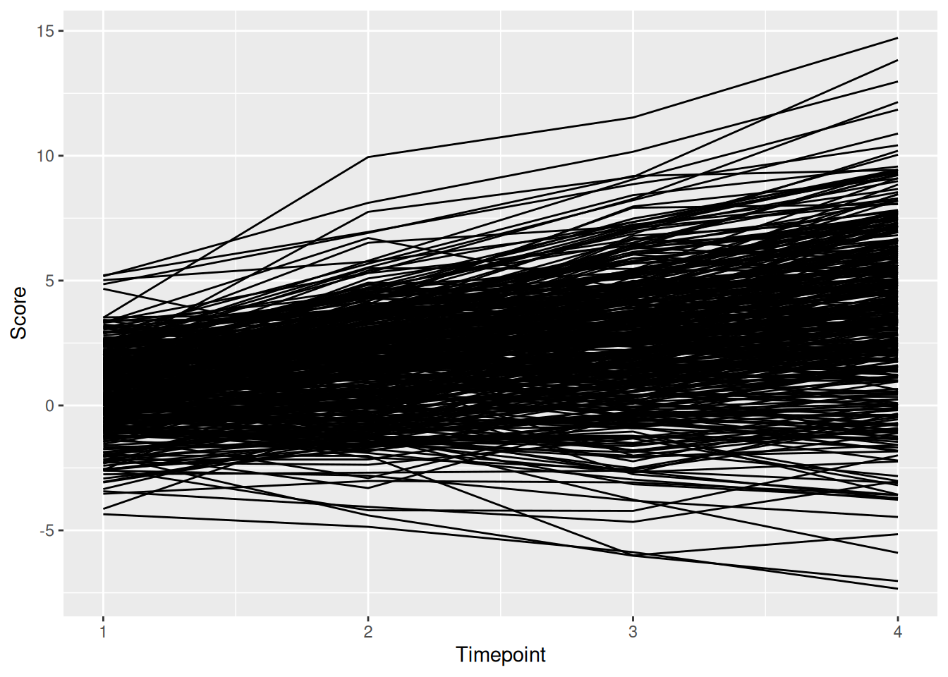
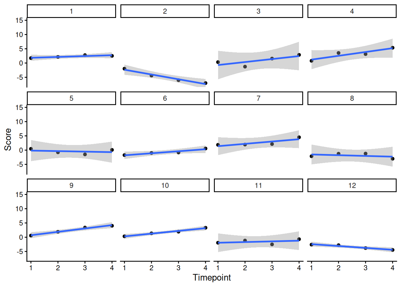
facetedPlots <- Demo.growth_long |>
ggplot(
aes(
x = timepoint,
y = score,
group = id
)
) +
geom_point() +
geom_smooth(
method = "lm"
) +
coord_cartesian(
ylim = c(min(Demo.growth_long$score, na.rm = TRUE), max(Demo.growth_long$score, na.rm = TRUE))) +
labs(
x = "Timepoint",
y = "Score"
) +
theme_classic() +
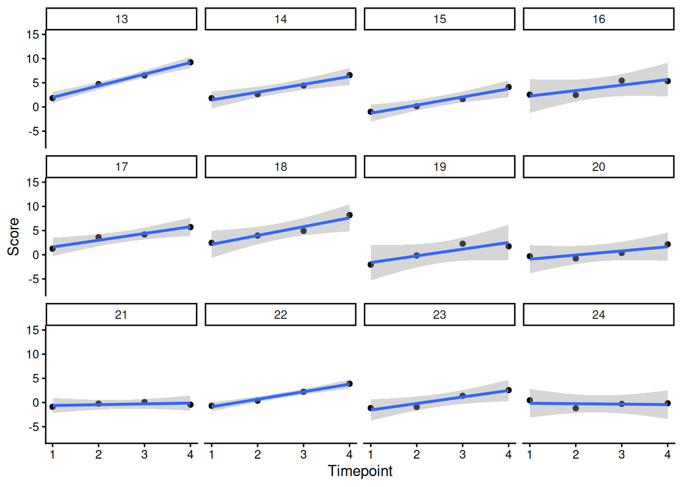
ggforce::facet_wrap_paginate(
~ id,
ncol = 4,
nrow = 3)
num_pages <- ggforce::n_pages(facetedPlots)for(i in 1:num_pages){
print(facetedPlots +
ggforce::facet_wrap_paginate(
~ id,
ncol = 4,
nrow = 3,
page = i))
}
See the chapter on latent growth curve modeling in lavaan: https://tdjorgensen.github.io/SEM-in-Ed-compendium/ch27.html (archived at https://perma.cc/C79K-BCLD).
For extensions, see the following resources:
lgcm1_syntax <- '
  # Intercept and slope
  intercept =~ 1*t1 + 1*t2 + 1*t3 + 1*t4
  slope =~ 0*t1 + 1*t2 + 2*t3 + 3*t4

  # Regression paths
  intercept ~ x1 + x2
  slope ~ x1 + x2

  # Time-varying covariates
  t1 ~ c1
  t2 ~ c2
  t3 ~ c3
  t4 ~ c4
'lgcm2_syntax <- '
# Intercept and slope
intercept =~ 1*t1 + 1*t2 + 1*t3 + 1*t4
slope =~ 0*t1 + 1*t2 + 2*t3 + 3*t4
# Regression paths
intercept ~ x1 + x2
slope ~ x1 + x2
# Time-varying covariates
t1 ~ c1
t2 ~ c2
t3 ~ c3
t4 ~ c4
# Constrain observed intercepts to zero
t1 ~ 0*1
t2 ~ 0*1
t3 ~ 0*1
t4 ~ 0*1
# Estimate mean of intercept and slope
intercept ~ 1
slope ~ 1
'lgcm1_fit <- growth(
lgcm1_syntax,
data = Demo.growth,
missing = "ML",
estimator = "MLR",
meanstructure = TRUE,
int.ov.free = FALSE,
int.lv.free = TRUE,
fixed.x = FALSE,
em.h1.iter.max = 100000)lgcm2_fit <- sem(
lgcm2_syntax,
data = Demo.growth,
missing = "ML",
estimator = "MLR",
meanstructure = TRUE,
fixed.x = FALSE,
em.h1.iter.max = 100000)summary(
lgcm1_fit,
fit.measures = TRUE,
standardized = TRUE,
rsquare = TRUE)lavaan 0.6-21 ended normally after 32 iterations
Estimator ML
Optimization method NLMINB
Number of model parameters 38
Number of observations 400
Number of missing patterns 1
Model Test User Model:
Standard Scaled
Test Statistic 40.774 40.982
Degrees of freedom 27 27
P-value (Chi-square) 0.043 0.041
Scaling correction factor 0.995
Yuan-Bentler correction (Mplus variant)
Model Test Baseline Model:
Test statistic 2345.885 2414.540
Degrees of freedom 30 30
P-value 0.000 0.000
Scaling correction factor 0.972
User Model versus Baseline Model:
Comparative Fit Index (CFI) 0.994 0.994
Tucker-Lewis Index (TLI) 0.993 0.993
Robust Comparative Fit Index (CFI) 0.992
Robust Tucker-Lewis Index (TLI) 0.992
Loglikelihood and Information Criteria:
Loglikelihood user model (H0) -5782.507 -5782.507
Scaling correction factor 0.991
for the MLR correction
Loglikelihood unrestricted model (H1) -5762.120 -5762.120
Scaling correction factor 0.993
for the MLR correction
Akaike (AIC) 11641.014 11641.014
Bayesian (BIC) 11792.690 11792.690
Sample-size adjusted Bayesian (SABIC) 11672.114 11672.114
Root Mean Square Error of Approximation:
RMSEA 0.036 0.036
90 Percent confidence interval - lower 0.006 0.007
90 Percent confidence interval - upper 0.057 0.057
P-value H_0: RMSEA <= 0.050 0.854 0.849
P-value H_0: RMSEA >= 0.080 0.000 0.000
Robust RMSEA 0.040
90 Percent confidence interval - lower 0.019
90 Percent confidence interval - upper 0.059
P-value H_0: Robust RMSEA <= 0.050 0.793
P-value H_0: Robust RMSEA >= 0.080 0.000
Standardized Root Mean Square Residual:
SRMR 0.030 0.030
Parameter Estimates:
Standard errors Sandwich
Information bread Observed
Observed information based on Hessian
Latent Variables:
Estimate Std.Err z-value P(>|z|) Std.lv Std.all
intercept =~
t1 1.000 1.386 0.875
t2 1.000 1.386 0.660
t3 1.000 1.386 0.507
t4 1.000 1.386 0.411
slope =~
t1 0.000 0.000 0.000
t2 1.000 0.769 0.366
t3 2.000 1.539 0.562
t4 3.000 2.308 0.685
Regressions:
Estimate Std.Err z-value P(>|z|) Std.lv Std.all
intercept ~
x1 0.608 0.059 10.275 0.000 0.439 0.453
x2 0.604 0.062 9.776 0.000 0.436 0.423
slope ~
x1 0.262 0.029 8.968 0.000 0.341 0.352
x2 0.522 0.032 16.302 0.000 0.678 0.658
t1 ~
c1 0.143 0.045 3.198 0.001 0.143 0.089
t2 ~
c2 0.289 0.047 6.215 0.000 0.289 0.131
t3 ~
c3 0.328 0.047 7.011 0.000 0.328 0.112
t4 ~
c4 0.330 0.057 5.814 0.000 0.330 0.090
Covariances:
Estimate Std.Err z-value P(>|z|) Std.lv Std.all
.intercept ~~
.slope 0.075 0.040 1.890 0.059 0.152 0.152
x1 ~~
x2 0.141 0.050 2.798 0.005 0.141 0.140
c1 -0.039 0.051 -0.762 0.446 -0.039 -0.038
c2 0.023 0.048 0.493 0.622 0.023 0.024
c3 0.027 0.050 0.544 0.586 0.027 0.028
c4 -0.023 0.045 -0.519 0.604 -0.023 -0.024
x2 ~~
c1 -0.018 0.050 -0.358 0.721 -0.018 -0.019
c2 -0.003 0.044 -0.075 0.940 -0.003 -0.004
c3 0.155 0.048 3.239 0.001 0.155 0.170
c4 -0.104 0.043 -2.421 0.015 -0.104 -0.116
c1 ~~
c2 0.080 0.045 1.793 0.073 0.080 0.086
c3 -0.030 0.050 -0.585 0.559 -0.030 -0.032
c4 0.127 0.048 2.668 0.008 0.127 0.140
c2 ~~
c3 0.003 0.041 0.078 0.938 0.003 0.004
c4 0.031 0.044 0.715 0.475 0.031 0.036
c3 ~~
c4 0.034 0.044 0.767 0.443 0.034 0.039
Intercepts:
Estimate Std.Err z-value P(>|z|) Std.lv Std.all
.intercept 0.580 0.061 9.501 0.000 0.419 0.419
.slope 0.958 0.030 32.177 0.000 1.244 1.244
Variances:
Estimate Std.Err z-value P(>|z|) Std.lv Std.all
.t1 0.580 0.091 6.386 0.000 0.580 0.231
.t2 0.596 0.056 10.627 0.000 0.596 0.135
.t3 0.481 0.051 9.434 0.000 0.481 0.064
.t4 0.535 0.094 5.709 0.000 0.535 0.047
.intercept 1.079 0.108 9.996 0.000 0.562 0.562
.slope 0.224 0.027 8.373 0.000 0.378 0.378
x1 1.064 0.068 15.614 0.000 1.064 1.000
x2 0.943 0.065 14.401 0.000 0.943 1.000
c1 0.972 0.064 15.306 0.000 0.972 1.000
c2 0.900 0.063 14.372 0.000 0.900 1.000
c3 0.876 0.067 13.041 0.000 0.876 1.000
c4 0.852 0.057 15.005 0.000 0.852 1.000
R-Square:
Estimate
t1 0.769
t2 0.865
t3 0.936
t4 0.953
intercept 0.438
slope 0.622summary(
lgcm2_fit,
fit.measures = TRUE,
standardized = TRUE,
rsquare = TRUE)lavaan 0.6-21 ended normally after 31 iterations
Estimator ML
Optimization method NLMINB
Number of model parameters 44
Number of observations 400
Number of missing patterns 1
Model Test User Model:
Standard Scaled
Test Statistic 26.059 26.344
Degrees of freedom 21 21
P-value (Chi-square) 0.204 0.194
Scaling correction factor 0.989
Yuan-Bentler correction (Mplus variant)
Model Test Baseline Model:
Test statistic 2345.885 2414.540
Degrees of freedom 30 30
P-value 0.000 0.000
Scaling correction factor 0.972
User Model versus Baseline Model:
Comparative Fit Index (CFI) 0.998 0.998
Tucker-Lewis Index (TLI) 0.997 0.997
Robust Comparative Fit Index (CFI) 0.998
Robust Tucker-Lewis Index (TLI) 0.997
Loglikelihood and Information Criteria:
Loglikelihood user model (H0) -5775.149 -5775.149
Scaling correction factor 0.994
for the MLR correction
Loglikelihood unrestricted model (H1) -5762.120 -5762.120
Scaling correction factor 0.993
for the MLR correction
Akaike (AIC) 11638.299 11638.299
Bayesian (BIC) 11813.923 11813.923
Sample-size adjusted Bayesian (SABIC) 11674.308 11674.308
Root Mean Square Error of Approximation:
RMSEA 0.025 0.025
90 Percent confidence interval - lower 0.000 0.000
90 Percent confidence interval - upper 0.051 0.052
P-value H_0: RMSEA <= 0.050 0.938 0.933
P-value H_0: RMSEA >= 0.080 0.000 0.000
Robust RMSEA 0.024
90 Percent confidence interval - lower 0.000
90 Percent confidence interval - upper 0.051
P-value H_0: Robust RMSEA <= 0.050 0.940
P-value H_0: Robust RMSEA >= 0.080 0.000
Standardized Root Mean Square Residual:
SRMR 0.014 0.014
Parameter Estimates:
Standard errors Sandwich
Information bread Observed
Observed information based on Hessian
Latent Variables:
Estimate Std.Err z-value P(>|z|) Std.lv Std.all
intercept =~
t1 1.000 1.386 0.875
t2 1.000 1.386 0.660
t3 1.000 1.386 0.507
t4 1.000 1.386 0.412
slope =~
t1 0.000 0.000 0.000
t2 1.000 0.768 0.366
t3 2.000 1.536 0.562
t4 3.000 2.304 0.684
Regressions:
Estimate Std.Err z-value P(>|z|) Std.lv Std.all
intercept ~
x1 0.608 0.059 10.275 0.000 0.439 0.451
x2 0.604 0.062 9.776 0.000 0.436 0.419
slope ~
x1 0.262 0.029 8.968 0.000 0.341 0.351
x2 0.522 0.032 16.301 0.000 0.679 0.653
t1 ~
c1 0.143 0.045 3.198 0.001 0.143 0.089
t2 ~
c2 0.289 0.047 6.215 0.000 0.289 0.131
t3 ~
c3 0.328 0.047 7.011 0.000 0.328 0.112
t4 ~
c4 0.330 0.057 5.814 0.000 0.330 0.091
Covariances:
Estimate Std.Err z-value P(>|z|) Std.lv Std.all
.intercept ~~
.slope 0.075 0.040 1.890 0.059 0.152 0.152
x1 ~~
x2 0.153 0.049 3.129 0.002 0.153 0.155
c1 -0.038 0.050 -0.760 0.447 -0.038 -0.037
c2 0.026 0.048 0.547 0.585 0.026 0.027
c3 0.033 0.049 0.674 0.501 0.033 0.035
c4 -0.025 0.044 -0.560 0.575 -0.025 -0.026
x2 ~~
c1 -0.019 0.050 -0.377 0.706 -0.019 -0.020
c2 -0.007 0.044 -0.167 0.867 -0.007 -0.008
c3 0.145 0.048 3.055 0.002 0.145 0.162
c4 -0.102 0.043 -2.371 0.018 -0.102 -0.115
c1 ~~
c2 0.080 0.045 1.789 0.074 0.080 0.085
c3 -0.030 0.050 -0.596 0.551 -0.030 -0.033
c4 0.128 0.048 2.669 0.008 0.128 0.140
c2 ~~
c3 0.001 0.042 0.030 0.976 0.001 0.001
c4 0.032 0.044 0.729 0.466 0.032 0.036
c3 ~~
c4 0.035 0.044 0.796 0.426 0.035 0.041
Intercepts:
Estimate Std.Err z-value P(>|z|) Std.lv Std.all
.t1 0.000 0.000 0.000
.t2 0.000 0.000 0.000
.t3 0.000 0.000 0.000
.t4 0.000 0.000 0.000
.intercept 0.580 0.061 9.501 0.000 0.419 0.419
.slope 0.958 0.030 32.177 0.000 1.247 1.247
x1 -0.092 0.051 -1.793 0.073 -0.092 -0.090
x2 0.138 0.048 2.878 0.004 0.138 0.144
c1 0.008 0.049 0.158 0.874 0.008 0.008
c2 0.029 0.047 0.610 0.542 0.029 0.031
c3 0.068 0.047 1.449 0.147 0.068 0.072
c4 -0.018 0.046 -0.390 0.696 -0.018 -0.020
Variances:
Estimate Std.Err z-value P(>|z|) Std.lv Std.all
.t1 0.580 0.091 6.386 0.000 0.580 0.231
.t2 0.596 0.056 10.627 0.000 0.596 0.135
.t3 0.481 0.051 9.434 0.000 0.481 0.064
.t4 0.535 0.094 5.709 0.000 0.535 0.047
.intercept 1.079 0.108 9.996 0.000 0.562 0.562
.slope 0.224 0.027 8.373 0.000 0.379 0.379
x1 1.056 0.068 15.511 0.000 1.056 1.000
x2 0.924 0.065 14.153 0.000 0.924 1.000
c1 0.972 0.063 15.321 0.000 0.972 1.000
c2 0.899 0.062 14.432 0.000 0.899 1.000
c3 0.872 0.067 13.018 0.000 0.872 1.000
c4 0.851 0.057 15.001 0.000 0.851 1.000
R-Square:
Estimate
t1 0.769
t2 0.865
t3 0.936
t4 0.953
intercept 0.438
slope 0.621fitMeasures(
lgcm1_fit,
fit.measures = c(
"chisq", "df", "pvalue",
"chisq.scaled", "df.scaled", "pvalue.scaled",
"chisq.scaling.factor",
"baseline.chisq","baseline.df","baseline.pvalue",
"rmsea", "cfi", "tli", "srmr",
"rmsea.robust", "cfi.robust", "tli.robust")) chisq df pvalue
40.774 27.000 0.043
chisq.scaled df.scaled pvalue.scaled
40.982 27.000 0.041
chisq.scaling.factor baseline.chisq baseline.df
0.995 2345.885 30.000
baseline.pvalue rmsea cfi
0.000 0.036 0.994
tli srmr rmsea.robust
0.993 0.030 0.040
cfi.robust tli.robust
0.992 0.992 residuals(
lgcm1_fit,
type = "cor")$type
[1] "cor.bollen"
$cov
t1 t2 t3 t4 x1 x2 c1 c2 c3 c4
t1 0.000
t2 0.010 0.000
t3 -0.013 -0.001 0.000
t4 0.012 0.002 0.002 0.000
x1 0.007 0.004 0.002 0.010 0.000
x2 -0.006 0.005 0.002 -0.002 0.015 0.000
c1 0.006 0.018 0.001 0.056 0.001 -0.001 0.000
c2 0.006 -0.005 -0.007 -0.005 0.003 -0.004 0.000 0.000
c3 0.046 0.018 0.030 0.030 0.007 -0.008 -0.001 -0.002 0.000
c4 0.038 0.027 0.001 0.006 -0.002 0.002 0.000 0.001 0.002 0.000
$mean
t1 t2 t3 t4 x1 x2 c1 c2 c3 c4
0.009 0.064 0.036 0.055 -0.090 0.144 0.008 0.031 0.072 -0.020 modificationindices(
lgcm1_fit,
sort. = TRUE)compRelSEM(lgcm1_fit)Error in `PHI[[b.idx]][myFacNames, myFacNames, drop = FALSE]`:
! subscript out of boundssemPlot::semPaths(
lgcm1_fit,
what = "Std.all",
layout = "tree2",
edge.label.cex = 1.5)
lavaanPlot::lavaanPlot(
  lgcm1_fit,
  coefs = TRUE,
  #covs = TRUE,
stand = TRUE)lavaanPlot::lavaanPlot2(
lgcm1_fit,
#stand = TRUE, # currently throws error; uncomment out when fixed: https://github.com/alishinski/lavaanPlot/issues/52
coef_labels = TRUE)To generate an interactive/modifiable path diagram, you can use the following syntax:
lavaangui::plot_lavaan(lgcm1_fit)lgcm1_intercept <- coef(lgcm1_fit)["intercept~1"]
lgcm1_slope <- coef(lgcm1_fit)["slope~1"]
timepoints <- 4
newData <- expand.grid(
time = c(1, 4)
)
newData$predictedValue <- NA
newData$predictedValue[which(newData$time == 1)] <- lgcm1_intercept
newData$predictedValue[which(newData$time == 4)] <- lgcm1_intercept + (timepoints - 1)*lgcm1_slope
ggplot(
data = newData,
mapping = aes(
x = time,
y = predictedValue)) +
geom_line(
linewidth = 1
) +
coord_cartesian(
ylim = c(0, 5)) +
labs(
x = "Timepoint",
y = "Score"
) +
theme_classic()
newData1 <- as.data.frame(predict(lgcm1_fit))
newData1$id <- row.names(newData1)

newData1$t1 <- newData1$intercept
newData1$t4 <- newData1$intercept + (timepoints - 1)*newData1$slope

newData2 <- pivot_longer(
  newData1,
  cols = c(t1, t4)) %>%
  select(-intercept, -slope)

newData2$time <- NA
newData2$time[which(newData2$name == "t1")] <- 1
newData2$time[which(newData2$name == "t4")] <- 4

ggplot(
  data = newData2,
  mapping = aes(
    x = time,
    y = value,
    group = factor(id))) +
  geom_line() +
  labs(
    x = "Timepoint",
    y = "Score"
  ) +
   theme_classic()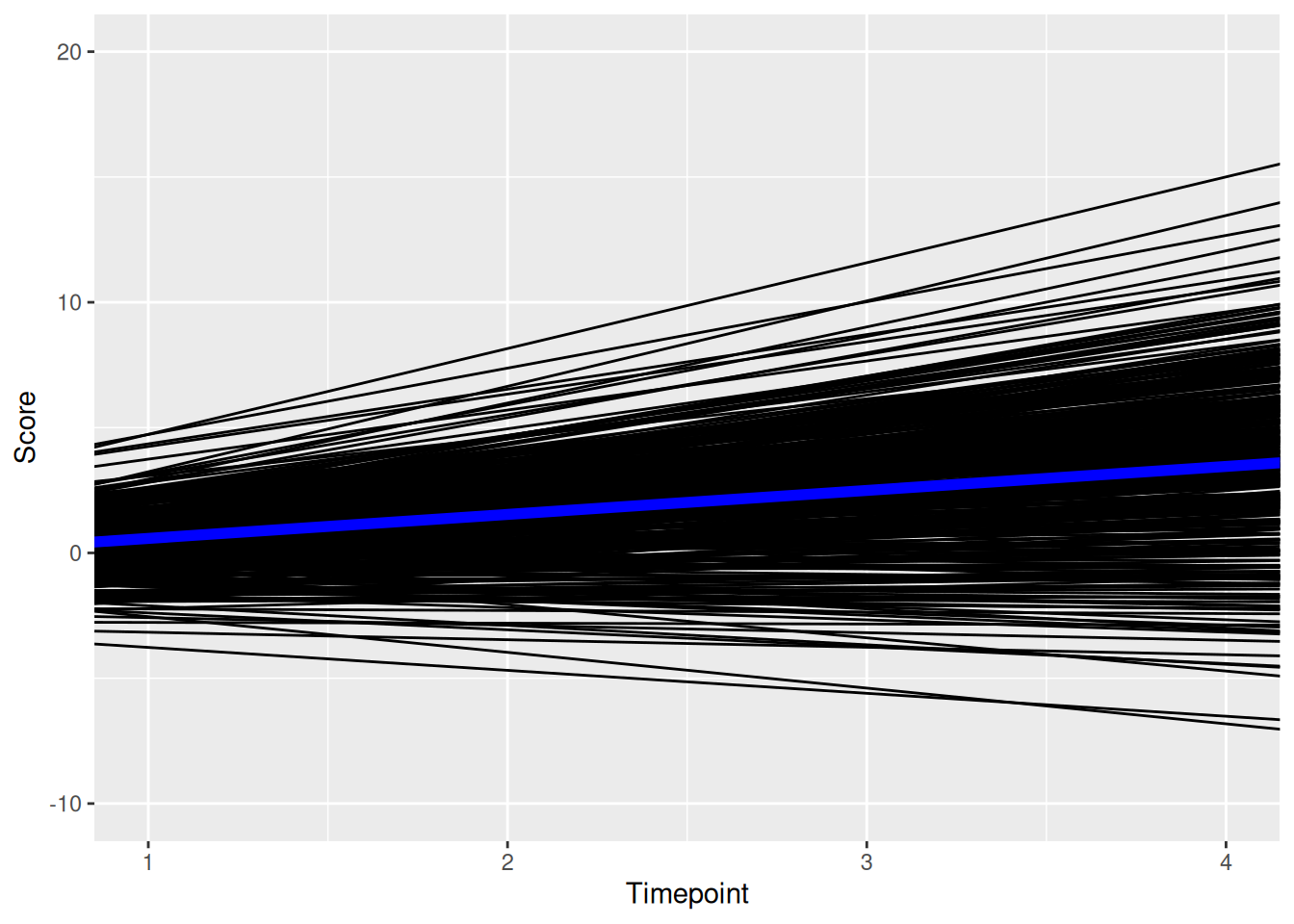
ggplot() +
  geom_line( # individuals' trajectories
    data = newData2,
    mapping = aes(
      x = time,
      y = value,
    group = factor(id)),
    color = "gray",
    alpha = 0.5
  ) +
  geom_line( # prototypical trajectory
    data = newData,
    mapping = aes(
      x = time,
      y = predictedValue
    ),
    linewidth = 2
  ) +
  labs(
    x = "Timepoint",
    y = "Score"
  ) +
   theme_classic()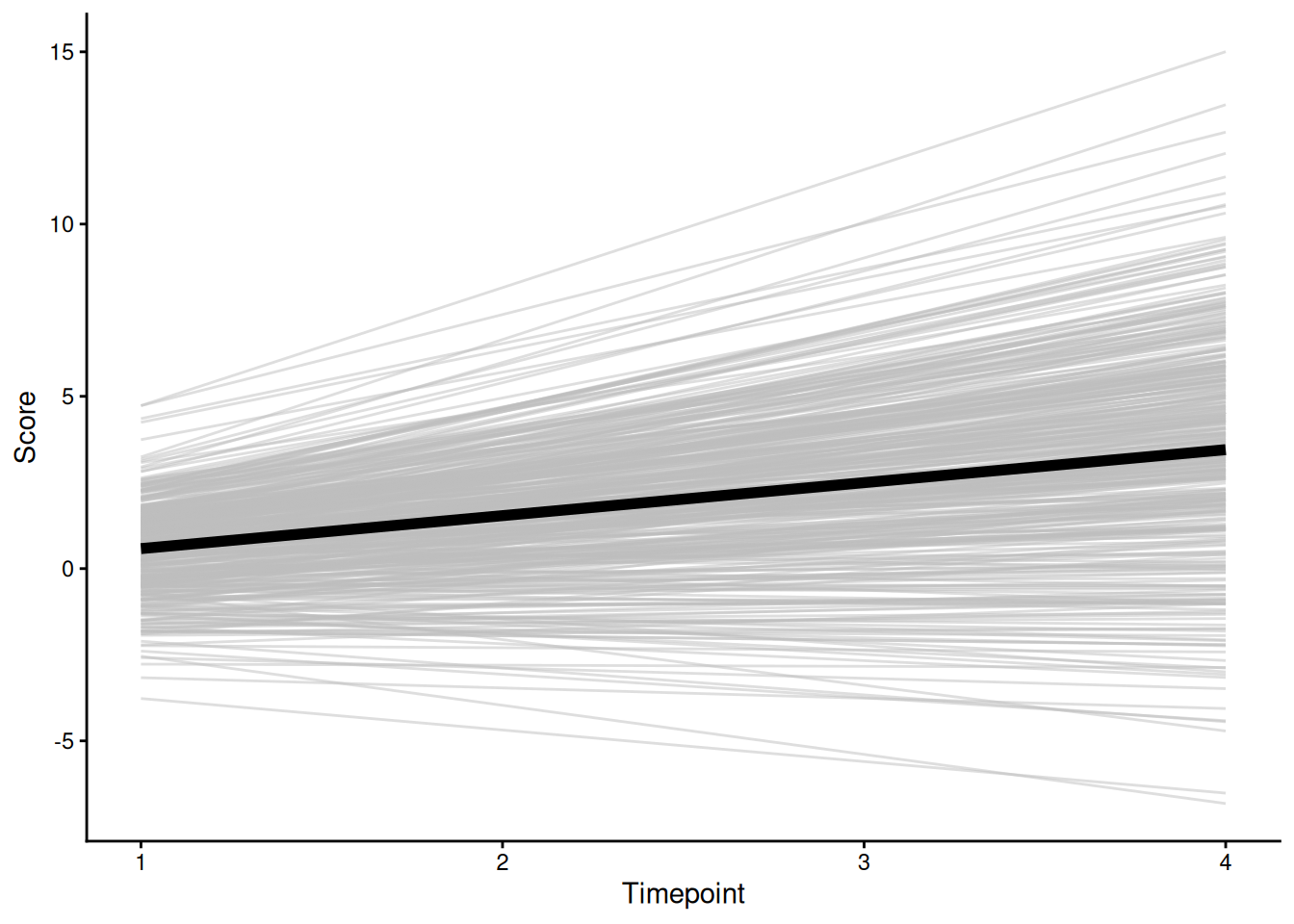
lbgcm1_syntax <- '
  # Intercept and slope
  intercept =~ 1*t1 + 1*t2 + 1*t3 + 1*t4
  slope =~ 0*t1 + a*t2 + b*t3 + 1*t4 # freely estimate the loadings for t2 and t3

  # Regression paths
  intercept ~ x1 + x2
  slope ~ x1 + x2

  # Time-varying covariates
  t1 ~ c1
  t2 ~ c2
  t3 ~ c3
  t4 ~ c4
'lbgcm2_syntax <- '
# Intercept and slope
intercept =~ 1*t1 + 1*t2 + 1*t3 + 1*t4
slope =~ 0*t1 + a*t2 + b*t3 + 1*t4 # freely estimate the loadings for t2 and t3
# Regression paths
intercept ~ x1 + x2
slope ~ x1 + x2
# Time-varying covariates
t1 ~ c1
t2 ~ c2
t3 ~ c3
t4 ~ c4
# Constrain observed intercepts to zero
t1 ~ 0*1
t2 ~ 0*1
t3 ~ 0*1
t4 ~ 0*1
# Estimate mean of intercept and slope
intercept ~ 1
slope ~ 1
'lbgcm1_fit <- growth(
lbgcm1_syntax,
data = Demo.growth,
missing = "ML",
estimator = "MLR",
meanstructure = TRUE,
int.ov.free = FALSE,
int.lv.free = TRUE,
fixed.x = FALSE,
em.h1.iter.max = 100000)lbgcm2_fit <- sem(
lbgcm2_syntax,
data = Demo.growth,
missing = "ML",
estimator = "MLR",
meanstructure = TRUE,
fixed.x = FALSE,
em.h1.iter.max = 100000)summary(
lbgcm1_fit,
fit.measures = TRUE,
standardized = TRUE,
rsquare = TRUE)lavaan 0.6-21 ended normally after 42 iterations
Estimator ML
Optimization method NLMINB
Number of model parameters 40
Number of observations 400
Number of missing patterns 1
Model Test User Model:
Standard Scaled
Test Statistic 37.229 37.400
Degrees of freedom 25 25
P-value (Chi-square) 0.055 0.053
Scaling correction factor 0.995
Yuan-Bentler correction (Mplus variant)
Model Test Baseline Model:
Test statistic 2345.885 2414.540
Degrees of freedom 30 30
P-value 0.000 0.000
Scaling correction factor 0.972
User Model versus Baseline Model:
Comparative Fit Index (CFI) 0.995 0.995
Tucker-Lewis Index (TLI) 0.994 0.994
Robust Comparative Fit Index (CFI) 0.993
Robust Tucker-Lewis Index (TLI) 0.992
Loglikelihood and Information Criteria:
Loglikelihood user model (H0) -5780.735 -5780.735
Scaling correction factor 0.991
for the MLR correction
Loglikelihood unrestricted model (H1) -5762.120 -5762.120
Scaling correction factor 0.993
for the MLR correction
Akaike (AIC) 11641.470 11641.470
Bayesian (BIC) 11801.128 11801.128
Sample-size adjusted Bayesian (SABIC) 11674.206 11674.206
Root Mean Square Error of Approximation:
RMSEA 0.035 0.035
90 Percent confidence interval - lower 0.000 0.000
90 Percent confidence interval - upper 0.057 0.057
P-value H_0: RMSEA <= 0.050 0.855 0.851
P-value H_0: RMSEA >= 0.080 0.000 0.000
Robust RMSEA 0.040
90 Percent confidence interval - lower 0.018
90 Percent confidence interval - upper 0.059
P-value H_0: Robust RMSEA <= 0.050 0.793
P-value H_0: Robust RMSEA >= 0.080 0.000
Standardized Root Mean Square Residual:
SRMR 0.029 0.029
Parameter Estimates:
Standard errors Sandwich
Information bread Observed
Observed information based on Hessian
Latent Variables:
Estimate Std.Err z-value P(>|z|) Std.lv Std.all
intercept =~
t1 1.000 1.381 0.875
t2 1.000 1.381 0.650
t3 1.000 1.381 0.508
t4 1.000 1.381 0.409
slope =~
t1 0.000 0.000 0.000
t2 (a) 0.348 0.013 26.867 0.000 0.811 0.382
t3 (b) 0.653 0.012 53.301 0.000 1.523 0.561
t4 1.000 2.330 0.690
Regressions:
Estimate Std.Err z-value P(>|z|) Std.lv Std.all
intercept ~
x1 0.605 0.059 10.192 0.000 0.438 0.452
x2 0.598 0.062 9.619 0.000 0.433 0.420
slope ~
x1 0.794 0.089 8.969 0.000 0.341 0.351
x2 1.578 0.097 16.223 0.000 0.677 0.657
t1 ~
c1 0.145 0.045 3.226 0.001 0.145 0.090
t2 ~
c2 0.287 0.047 6.157 0.000 0.287 0.128
t3 ~
c3 0.337 0.047 7.111 0.000 0.337 0.116
t4 ~
c4 0.333 0.057 5.836 0.000 0.333 0.091
Covariances:
Estimate Std.Err z-value P(>|z|) Std.lv Std.all
.intercept ~~
.slope 0.215 0.120 1.790 0.074 0.144 0.144
x1 ~~
x2 0.141 0.050 2.798 0.005 0.141 0.140
c1 -0.039 0.051 -0.762 0.446 -0.039 -0.038
c2 0.023 0.048 0.493 0.622 0.023 0.024
c3 0.027 0.050 0.544 0.586 0.027 0.028
c4 -0.023 0.045 -0.519 0.604 -0.023 -0.024
x2 ~~
c1 -0.018 0.050 -0.358 0.721 -0.018 -0.019
c2 -0.003 0.044 -0.075 0.940 -0.003 -0.004
c3 0.155 0.048 3.239 0.001 0.155 0.170
c4 -0.104 0.043 -2.421 0.015 -0.104 -0.116
c1 ~~
c2 0.080 0.045 1.793 0.073 0.080 0.086
c3 -0.030 0.050 -0.585 0.559 -0.030 -0.032
c4 0.127 0.048 2.668 0.008 0.127 0.140
c2 ~~
c3 0.003 0.041 0.078 0.938 0.003 0.004
c4 0.031 0.044 0.715 0.475 0.031 0.036
c3 ~~
c4 0.034 0.044 0.767 0.443 0.034 0.039
Intercepts:
Estimate Std.Err z-value P(>|z|) Std.lv Std.all
.intercept 0.568 0.063 8.966 0.000 0.411 0.411
.slope 2.899 0.091 31.916 0.000 1.244 1.244
Variances:
Estimate Std.Err z-value P(>|z|) Std.lv Std.all
.t1 0.574 0.092 6.211 0.000 0.574 0.230
.t2 0.595 0.055 10.741 0.000 0.595 0.132
.t3 0.487 0.051 9.602 0.000 0.487 0.066
.t4 0.518 0.097 5.338 0.000 0.518 0.045
.intercept 1.079 0.109 9.932 0.000 0.566 0.566
.slope 2.060 0.246 8.388 0.000 0.379 0.379
x1 1.064 0.068 15.614 0.000 1.064 1.000
x2 0.943 0.065 14.401 0.000 0.943 1.000
c1 0.972 0.064 15.306 0.000 0.972 1.000
c2 0.900 0.063 14.372 0.000 0.900 1.000
c3 0.876 0.067 13.041 0.000 0.876 1.000
c4 0.852 0.057 15.005 0.000 0.852 1.000
R-Square:
Estimate
t1 0.770
t2 0.868
t3 0.934
t4 0.955
intercept 0.434
slope 0.621summary(
lbgcm2_fit,
fit.measures = TRUE,
standardized = TRUE,
rsquare = TRUE)lavaan 0.6-21 ended normally after 43 iterations
Estimator ML
Optimization method NLMINB
Number of model parameters 46
Number of observations 400
Number of missing patterns 1
Model Test User Model:
Standard Scaled
Test Statistic 22.514 22.759
Degrees of freedom 19 19
P-value (Chi-square) 0.259 0.248
Scaling correction factor 0.989
Yuan-Bentler correction (Mplus variant)
Model Test Baseline Model:
Test statistic 2345.885 2414.540
Degrees of freedom 30 30
P-value 0.000 0.000
Scaling correction factor 0.972
User Model versus Baseline Model:
Comparative Fit Index (CFI) 0.998 0.998
Tucker-Lewis Index (TLI) 0.998 0.998
Robust Comparative Fit Index (CFI) 0.999
Robust Tucker-Lewis Index (TLI) 0.998
Loglikelihood and Information Criteria:
Loglikelihood user model (H0) -5773.377 -5773.377
Scaling correction factor 0.994
for the MLR correction
Loglikelihood unrestricted model (H1) -5762.120 -5762.120
Scaling correction factor 0.993
for the MLR correction
Akaike (AIC) 11638.754 11638.754
Bayesian (BIC) 11822.361 11822.361
Sample-size adjusted Bayesian (SABIC) 11676.400 11676.400
Root Mean Square Error of Approximation:
RMSEA 0.022 0.022
90 Percent confidence interval - lower 0.000 0.000
90 Percent confidence interval - upper 0.051 0.051
P-value H_0: RMSEA <= 0.050 0.944 0.939
P-value H_0: RMSEA >= 0.080 0.000 0.000
Robust RMSEA 0.021
90 Percent confidence interval - lower 0.000
90 Percent confidence interval - upper 0.051
P-value H_0: Robust RMSEA <= 0.050 0.945
P-value H_0: Robust RMSEA >= 0.080 0.000
Standardized Root Mean Square Residual:
SRMR 0.013 0.013
Parameter Estimates:
Standard errors Sandwich
Information bread Observed
Observed information based on Hessian
Latent Variables:
Estimate Std.Err z-value P(>|z|) Std.lv Std.all
intercept =~
t1 1.000 1.381 0.875
t2 1.000 1.381 0.651
t3 1.000 1.381 0.509
t4 1.000 1.381 0.409
slope =~
t1 0.000 0.000 0.000
t2 (a) 0.348 0.013 26.867 0.000 0.809 0.381
t3 (b) 0.653 0.012 53.301 0.000 1.520 0.560
t4 1.000 2.326 0.689
Regressions:
Estimate Std.Err z-value P(>|z|) Std.lv Std.all
intercept ~
x1 0.605 0.059 10.192 0.000 0.438 0.450
x2 0.598 0.062 9.619 0.000 0.433 0.416
slope ~
x1 0.794 0.089 8.969 0.000 0.341 0.351
x2 1.578 0.097 16.223 0.000 0.678 0.652
t1 ~
c1 0.145 0.045 3.226 0.001 0.145 0.090
t2 ~
c2 0.287 0.047 6.157 0.000 0.287 0.128
t3 ~
c3 0.337 0.047 7.111 0.000 0.337 0.116
t4 ~
c4 0.333 0.057 5.836 0.000 0.333 0.091
Covariances:
Estimate Std.Err z-value P(>|z|) Std.lv Std.all
.intercept ~~
.slope 0.215 0.120 1.790 0.074 0.144 0.144
x1 ~~
x2 0.153 0.049 3.129 0.002 0.153 0.155
c1 -0.038 0.050 -0.760 0.447 -0.038 -0.037
c2 0.026 0.048 0.547 0.585 0.026 0.027
c3 0.033 0.049 0.674 0.501 0.033 0.035
c4 -0.025 0.044 -0.560 0.575 -0.025 -0.026
x2 ~~
c1 -0.019 0.050 -0.377 0.706 -0.019 -0.020
c2 -0.007 0.044 -0.167 0.867 -0.007 -0.008
c3 0.145 0.048 3.055 0.002 0.145 0.162
c4 -0.102 0.043 -2.371 0.018 -0.102 -0.115
c1 ~~
c2 0.080 0.045 1.789 0.074 0.080 0.085
c3 -0.030 0.050 -0.596 0.551 -0.030 -0.033
c4 0.128 0.048 2.669 0.008 0.128 0.140
c2 ~~
c3 0.001 0.042 0.030 0.976 0.001 0.001
c4 0.032 0.044 0.729 0.466 0.032 0.036
c3 ~~
c4 0.035 0.044 0.796 0.426 0.035 0.041
Intercepts:
Estimate Std.Err z-value P(>|z|) Std.lv Std.all
.t1 0.000 0.000 0.000
.t2 0.000 0.000 0.000
.t3 0.000 0.000 0.000
.t4 0.000 0.000 0.000
.intercept 0.568 0.063 8.966 0.000 0.411 0.411
.slope 2.899 0.091 31.916 0.000 1.246 1.246
x1 -0.092 0.051 -1.793 0.073 -0.092 -0.090
x2 0.138 0.048 2.878 0.004 0.138 0.144
c1 0.008 0.049 0.158 0.874 0.008 0.008
c2 0.029 0.047 0.610 0.542 0.029 0.031
c3 0.068 0.047 1.449 0.147 0.068 0.072
c4 -0.018 0.046 -0.390 0.696 -0.018 -0.020
Variances:
Estimate Std.Err z-value P(>|z|) Std.lv Std.all
.t1 0.574 0.092 6.211 0.000 0.574 0.230
.t2 0.595 0.055 10.741 0.000 0.595 0.132
.t3 0.487 0.051 9.602 0.000 0.487 0.066
.t4 0.518 0.097 5.338 0.000 0.518 0.046
.intercept 1.079 0.109 9.932 0.000 0.566 0.566
.slope 2.060 0.246 8.388 0.000 0.381 0.381
x1 1.056 0.068 15.511 0.000 1.056 1.000
x2 0.924 0.065 14.153 0.000 0.924 1.000
c1 0.972 0.063 15.321 0.000 0.972 1.000
c2 0.899 0.062 14.432 0.000 0.899 1.000
c3 0.872 0.067 13.018 0.000 0.872 1.000
c4 0.851 0.057 15.001 0.000 0.851 1.000
R-Square:
Estimate
t1 0.770
t2 0.868
t3 0.934
t4 0.954
intercept 0.434
slope 0.619fitMeasures(
lbgcm1_fit,
fit.measures = c(
"chisq", "df", "pvalue",
"chisq.scaled", "df.scaled", "pvalue.scaled",
"chisq.scaling.factor",
"baseline.chisq","baseline.df","baseline.pvalue",
"rmsea", "cfi", "tli", "srmr",
"rmsea.robust", "cfi.robust", "tli.robust")) chisq df pvalue
37.229 25.000 0.055
chisq.scaled df.scaled pvalue.scaled
37.400 25.000 0.053
chisq.scaling.factor baseline.chisq baseline.df
0.995 2345.885 30.000
baseline.pvalue rmsea cfi
0.000 0.035 0.995
tli srmr rmsea.robust
0.994 0.029 0.040
cfi.robust tli.robust
0.993 0.992 residuals(
lbgcm1_fit,
type = "cor")$type
[1] "cor.bollen"
$cov
t1 t2 t3 t4 x1 x2 c1 c2 c3 c4
t1 0.000
t2 0.012 0.000
t3 -0.011 -0.003 0.000
t4 0.016 -0.003 0.003 0.000
x1 0.008 0.003 0.003 0.009 0.000
x2 -0.003 0.001 0.004 -0.003 0.015 0.000
c1 0.004 0.018 0.001 0.056 0.001 -0.001 0.000
c2 0.006 -0.003 -0.007 -0.005 0.003 -0.004 0.000 0.000
c3 0.046 0.018 0.026 0.030 0.007 -0.008 -0.001 -0.002 0.000
c4 0.038 0.027 0.001 0.005 -0.002 0.002 0.000 0.001 0.002 0.000
$mean
t1 t2 t3 t4 x1 x2 c1 c2 c3 c4
0.017 0.046 0.048 0.051 -0.090 0.144 0.008 0.031 0.072 -0.020 modificationindices(
lbgcm1_fit,
sort. = TRUE)compRelSEM(lbgcm1_fit)Error in `PHI[[b.idx]][myFacNames, myFacNames, drop = FALSE]`:
! subscript out of boundssemPaths(
lbgcm1_fit,
what = "Std.all",
layout = "tree2",
edge.label.cex = 1.5)
lavaanPlot::lavaanPlot(
  lbgcm1_fit,
  coefs = TRUE,
  #covs = TRUE,
stand = TRUE)lavaanPlot::lavaanPlot2(
lbgcm1_fit,
stand = TRUE,
coef_labels = TRUE)To generate an interactive/modifiable path diagram, you can use the following syntax:
lavaangui::plot_lavaan(lbgcm1_fit)lbgcm1_intercept <- coef(lbgcm1_fit)["intercept~1"]
lbgcm1_slope <- coef(lbgcm1_fit)["slope~1"]
lbgcm1_slopeloadingt2 <- coef(lbgcm1_fit)["a"]
lbgcm1_slopeloadingt3 <- coef(lbgcm1_fit)["b"]
timepoints <- 4
newData <- data.frame(
time = 1:4,
slopeloading = c(0, lbgcm1_slopeloadingt2, lbgcm1_slopeloadingt3, 1)
)
newData$predictedValue <- NA
newData$predictedValue <- lbgcm1_intercept + lbgcm1_slope * newData$slopeloading
ggplot(
data = newData,
mapping = aes(
x = time,
y = predictedValue)) +
geom_line(
linewidth = 1
) +
coord_cartesian(
ylim = c(0, 5)) +
labs(
x = "Timepoint",
y = "Score"
) +
theme_classic()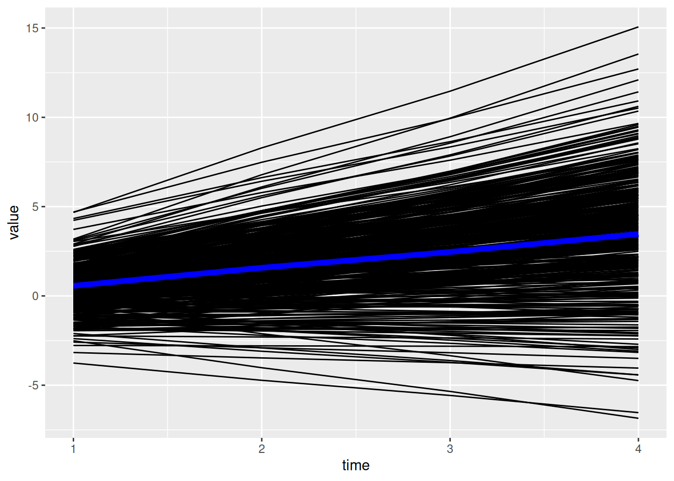
person_factors <- as.data.frame(predict(lbgcm1_fit))
person_factors$id <- rownames(person_factors)

slope_loadings <- c(0, lbgcm1_slopeloadingt2, lbgcm1_slopeloadingt3, 1)

# Compute model-implied values for each person at each time point
individual_trajectories <- person_factors %>%
  rowwise() %>%
  mutate(
    t1 = intercept + slope * slope_loadings[1],
    t2 = intercept + slope * slope_loadings[2],
    t3 = intercept + slope * slope_loadings[3],
    t4 = intercept + slope * slope_loadings[4]
  ) %>%
  ungroup() %>%
  select(id, t1, t2, t3, t4) %>%
  pivot_longer(
    cols = t1:t4,
    names_to = "timepoint",
    values_to = "value") %>%
  mutate(
    time = as.integer(substr(timepoint, 2, 2)) # extract number from "t1", "t2", etc.
  )

ggplot(
  data = individual_trajectories,
  mapping = aes(
    x = time,
    y = value,
    group = factor(id))) +
  geom_line() +
  labs(
    x = "Timepoint",
    y = "Score"
  ) +
   theme_classic()
ggplot() +
  geom_line( # individuals' model-implied trajectories
    data = individual_trajectories,
    aes(
      x = time,
      y = value,
      group = id),
    color = "gray",
    alpha = 0.5
  ) +
  geom_line( # prototypical trajectory
    data = newData,
    aes(
      x = time,
      y = predictedValue),
    color = "blue",
    linewidth = 2
  ) +
  labs(
    x = "Timepoint",
    y = "Score"
  ) +
   theme_classic()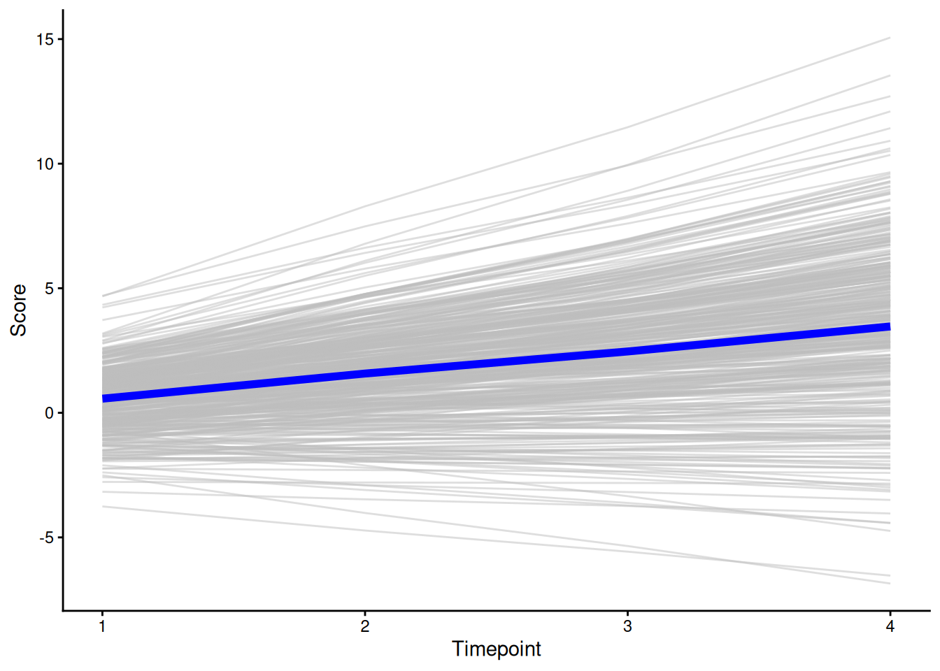
When using higher-order polynomials, we could specify contrast codes for time to reduce multicollinearity between the linear and quadratic growth factors: https://tdjorgensen.github.io/SEM-in-Ed-compendium/ch27.html#saturated-growth-model (archived at https://perma.cc/2CJX-WLLZ)
              1    2
[1,] -0.6708204  0.5
[2,] -0.2236068 -0.5
[3,]  0.2236068 -0.5
[4,]  0.6708204  0.5
attr(,"coefs")
attr(,"coefs")$alpha
[1] 1.5 1.5

attr(,"coefs")$norm2
[1] 1 4 5 4

attr(,"degree")
[1] 1 2
attr(,"class")
[1] "poly" "matrix"linearLoadings <- factorLoadings[,1]
quadraticLoadings <- factorLoadings[,2]
linearLoadings[1] -0.6708204 -0.2236068 0.2236068 0.6708204quadraticLoadings[1] 0.5 -0.5 -0.5 0.5quadraticGCM1_syntax <- '
# Intercept and slope
intercept =~ 1*t1 + 1*t2 + 1*t3 + 1*t4
linear =~ 0*t1 + 1*t2 + 2*t3 + 3*t4
quadratic =~ 0*t1 + 1*t2 + 4*t3 + 9*t4
# Regression paths
intercept ~ x1 + x2
linear ~ x1 + x2
quadratic ~ x1 + x2
# Time-varying covariates
t1 ~ c1
t2 ~ c2
t3 ~ c3
t4 ~ c4
'quadraticGCM2_syntax <- '
# Intercept and slope
intercept =~ 1*t1 + 1*t2 + 1*t3 + 1*t4
linear =~ 0*t1 + 1*t2 + 2*t3 + 3*t4
quadratic =~ 0*t1 + 1*t2 + 4*t3 + 9*t4
# Regression paths
intercept ~ x1 + x2
linear ~ x1 + x2
quadratic ~ x1 + x2
# Time-varying covariates
t1 ~ c1
t2 ~ c2
t3 ~ c3
t4 ~ c4
# Constrain observed intercepts to zero
t1 ~ 0*1
t2 ~ 0*1
t3 ~ 0*1
t4 ~ 0*1
# Estimate mean of intercept and slope
intercept ~ 1
linear ~ 1
quadratic ~ 1
'quadraticGCM1_fit <- growth(
quadraticGCM1_syntax,
data = Demo.growth,
missing = "ML",
estimator = "MLR",
meanstructure = TRUE,
int.ov.free = FALSE,
int.lv.free = TRUE,
fixed.x = FALSE,
em.h1.iter.max = 100000)quadraticGCM2_fit <- sem(
quadraticGCM2_syntax,
data = Demo.growth,
missing = "ML",
estimator = "MLR",
meanstructure = TRUE,
fixed.x = FALSE,
em.h1.iter.max = 100000)summary(
quadraticGCM1_fit,
fit.measures = TRUE,
standardized = TRUE,
rsquare = TRUE)lavaan 0.6-21 ended normally after 56 iterations
Estimator ML
Optimization method NLMINB
Number of model parameters 44
Number of observations 400
Number of missing patterns 1
Model Test User Model:
Standard Scaled
Test Statistic 35.756 35.604
Degrees of freedom 21 21
P-value (Chi-square) 0.023 0.024
Scaling correction factor 1.004
Yuan-Bentler correction (Mplus variant)
Model Test Baseline Model:
Test statistic 2345.885 2414.540
Degrees of freedom 30 30
P-value 0.000 0.000
Scaling correction factor 0.972
User Model versus Baseline Model:
Comparative Fit Index (CFI) 0.994 0.994
Tucker-Lewis Index (TLI) 0.991 0.991
Robust Comparative Fit Index (CFI) 0.992
Robust Tucker-Lewis Index (TLI) 0.989
Loglikelihood and Information Criteria:
Loglikelihood user model (H0) -5779.998 -5779.998
Scaling correction factor 0.987
for the MLR correction
Loglikelihood unrestricted model (H1) -5762.120 -5762.120
Scaling correction factor 0.993
for the MLR correction
Akaike (AIC) 11647.996 11647.996
Bayesian (BIC) 11823.621 11823.621
Sample-size adjusted Bayesian (SABIC) 11684.006 11684.006
Root Mean Square Error of Approximation:
RMSEA 0.042 0.042
90 Percent confidence interval - lower 0.016 0.015
90 Percent confidence interval - upper 0.065 0.065
P-value H_0: RMSEA <= 0.050 0.692 0.698
P-value H_0: RMSEA >= 0.080 0.002 0.002
Robust RMSEA 0.047
90 Percent confidence interval - lower 0.026
90 Percent confidence interval - upper 0.067
P-value H_0: Robust RMSEA <= 0.050 0.584
P-value H_0: Robust RMSEA >= 0.080 0.002
Standardized Root Mean Square Residual:
SRMR 0.030 0.030
Parameter Estimates:
Standard errors Sandwich
Information bread Observed
Observed information based on Hessian
Latent Variables:
Estimate Std.Err z-value P(>|z|) Std.lv Std.all
intercept =~
t1 1.000 1.509 0.956
t2 1.000 1.509 0.715
t3 1.000 1.509 0.553
t4 1.000 1.509 0.448
linear =~
t1 0.000 0.000 0.000
t2 1.000 1.054 0.499
t3 2.000 2.108 0.773
t4 3.000 3.163 0.938
quadratic =~
t1 0.000 0.000 0.000
t2 1.000 0.164 0.078
t3 4.000 0.655 0.240
t4 9.000 1.474 0.437
Regressions:
Estimate Std.Err z-value P(>|z|) Std.lv Std.all
intercept ~
x1 0.615 0.063 9.801 0.000 0.407 0.420
x2 0.590 0.066 8.878 0.000 0.391 0.380
linear ~
x1 0.236 0.063 3.737 0.000 0.224 0.231
x2 0.557 0.073 7.595 0.000 0.528 0.513
quadratic ~
x1 0.009 0.020 0.456 0.649 0.055 0.056
x2 -0.012 0.021 -0.549 0.583 -0.070 -0.068
t1 ~
c1 0.130 0.045 2.864 0.004 0.130 0.081
t2 ~
c2 0.289 0.047 6.207 0.000 0.289 0.130
t3 ~
c3 0.330 0.047 7.030 0.000 0.330 0.113
t4 ~
c4 0.326 0.057 5.726 0.000 0.326 0.089
Covariances:
Estimate Std.Err z-value P(>|z|) Std.lv Std.all
.intercept ~~
.linear -0.359 0.216 -1.658 0.097 -0.351 -0.351
.quadratic 0.108 0.053 2.025 0.043 0.552 0.552
.linear ~~
.quadratic -0.119 0.056 -2.121 0.034 -0.857 -0.857
x1 ~~
x2 0.141 0.050 2.798 0.005 0.141 0.140
c1 -0.039 0.051 -0.762 0.446 -0.039 -0.038
c2 0.023 0.048 0.493 0.622 0.023 0.024
c3 0.027 0.050 0.544 0.586 0.027 0.028
c4 -0.023 0.045 -0.519 0.604 -0.023 -0.024
x2 ~~
c1 -0.018 0.050 -0.358 0.721 -0.018 -0.019
c2 -0.003 0.044 -0.075 0.940 -0.003 -0.004
c3 0.155 0.048 3.239 0.001 0.155 0.170
c4 -0.104 0.043 -2.421 0.015 -0.104 -0.116
c1 ~~
c2 0.080 0.045 1.793 0.073 0.080 0.086
c3 -0.030 0.050 -0.585 0.559 -0.030 -0.032
c4 0.127 0.048 2.668 0.008 0.127 0.140
c2 ~~
c3 0.003 0.041 0.078 0.938 0.003 0.004
c4 0.031 0.044 0.715 0.475 0.031 0.036
c3 ~~
c4 0.034 0.044 0.767 0.443 0.034 0.039
Intercepts:
Estimate Std.Err z-value P(>|z|) Std.lv Std.all
.intercept 0.575 0.065 8.793 0.000 0.381 0.381
.linear 0.944 0.066 14.331 0.000 0.895 0.895
.quadratic 0.005 0.020 0.276 0.783 0.033 0.033
Variances:
Estimate Std.Err z-value P(>|z|) Std.lv Std.all
.t1 0.208 0.187 1.111 0.267 0.208 0.084
.t2 0.640 0.079 8.106 0.000 0.640 0.144
.t3 0.404 0.085 4.747 0.000 0.404 0.054
.t4 0.623 0.307 2.027 0.043 0.623 0.055
.intercept 1.445 0.208 6.939 0.000 0.635 0.635
.linear 0.723 0.229 3.160 0.002 0.650 0.650
.quadratic 0.027 0.020 1.353 0.176 0.993 0.993
x1 1.064 0.068 15.614 0.000 1.064 1.000
x2 0.943 0.065 14.401 0.000 0.943 1.000
c1 0.972 0.064 15.306 0.000 0.972 1.000
c2 0.900 0.063 14.372 0.000 0.900 1.000
c3 0.876 0.067 13.041 0.000 0.876 1.000
c4 0.852 0.057 15.005 0.000 0.852 1.000
R-Square:
Estimate
t1 0.916
t2 0.856
t3 0.946
t4 0.945
intercept 0.365
linear 0.350
quadratic 0.007summary(
quadraticGCM2_fit,
fit.measures = TRUE,
standardized = TRUE,
rsquare = TRUE)lavaan 0.6-21 ended normally after 56 iterations
Estimator ML
Optimization method NLMINB
Number of model parameters 50
Number of observations 400
Number of missing patterns 1
Model Test User Model:
Standard Scaled
Test Statistic 21.040 21.042
Degrees of freedom 15 15
P-value (Chi-square) 0.136 0.136
Scaling correction factor 1.000
Yuan-Bentler correction (Mplus variant)
Model Test Baseline Model:
Test statistic 2345.885 2414.540
Degrees of freedom 30 30
P-value 0.000 0.000
Scaling correction factor 0.972
User Model versus Baseline Model:
Comparative Fit Index (CFI) 0.997 0.997
Tucker-Lewis Index (TLI) 0.995 0.995
Robust Comparative Fit Index (CFI) 0.998
Robust Tucker-Lewis Index (TLI) 0.995
Loglikelihood and Information Criteria:
Loglikelihood user model (H0) -5772.640 -5772.640
Scaling correction factor 0.990
for the MLR correction
Loglikelihood unrestricted model (H1) -5762.120 -5762.120
Scaling correction factor 0.993
for the MLR correction
Akaike (AIC) 11645.281 11645.281
Bayesian (BIC) 11844.854 11844.854
Sample-size adjusted Bayesian (SABIC) 11686.201 11686.201
Root Mean Square Error of Approximation:
RMSEA 0.032 0.032
90 Percent confidence interval - lower 0.000 0.000
90 Percent confidence interval - upper 0.061 0.061
P-value H_0: RMSEA <= 0.050 0.828 0.828
P-value H_0: RMSEA >= 0.080 0.002 0.002
Robust RMSEA 0.031
90 Percent confidence interval - lower 0.000
90 Percent confidence interval - upper 0.061
P-value H_0: Robust RMSEA <= 0.050 0.834
P-value H_0: Robust RMSEA >= 0.080 0.002
Standardized Root Mean Square Residual:
SRMR 0.014 0.014
Parameter Estimates:
Standard errors Sandwich
Information bread Observed
Observed information based on Hessian
Latent Variables:
Estimate Std.Err z-value P(>|z|) Std.lv Std.all
intercept =~
t1 1.000 1.509 0.956
t2 1.000 1.509 0.715
t3 1.000 1.509 0.554
t4 1.000 1.509 0.448
linear =~
t1 0.000 0.000 0.000
t2 1.000 1.053 0.499
t3 2.000 2.106 0.773
t4 3.000 3.158 0.938
quadratic =~
t1 0.000 0.000 0.000
t2 1.000 0.164 0.078
t3 4.000 0.655 0.241
t4 9.000 1.474 0.438
Regressions:
Estimate Std.Err z-value P(>|z|) Std.lv Std.all
intercept ~
x1 0.615 0.063 9.801 0.000 0.407 0.419
x2 0.590 0.066 8.878 0.000 0.391 0.376
linear ~
x1 0.236 0.063 3.737 0.000 0.224 0.230
x2 0.557 0.073 7.595 0.000 0.529 0.508
quadratic ~
x1 0.009 0.020 0.456 0.649 0.055 0.056
x2 -0.012 0.021 -0.549 0.583 -0.070 -0.068
t1 ~
c1 0.130 0.045 2.864 0.004 0.130 0.081
t2 ~
c2 0.289 0.047 6.207 0.000 0.289 0.130
t3 ~
c3 0.330 0.047 7.030 0.000 0.330 0.113
t4 ~
c4 0.326 0.057 5.726 0.000 0.326 0.089
Covariances:
Estimate Std.Err z-value P(>|z|) Std.lv Std.all
.intercept ~~
.linear -0.359 0.216 -1.658 0.097 -0.351 -0.351
.quadratic 0.108 0.053 2.025 0.043 0.552 0.552
.linear ~~
.quadratic -0.119 0.056 -2.121 0.034 -0.857 -0.857
x1 ~~
x2 0.153 0.049 3.129 0.002 0.153 0.155
c1 -0.038 0.050 -0.760 0.447 -0.038 -0.037
c2 0.026 0.048 0.547 0.585 0.026 0.027
c3 0.033 0.049 0.674 0.501 0.033 0.035
c4 -0.025 0.044 -0.560 0.575 -0.025 -0.026
x2 ~~
c1 -0.019 0.050 -0.377 0.706 -0.019 -0.020
c2 -0.007 0.044 -0.167 0.867 -0.007 -0.008
c3 0.145 0.048 3.055 0.002 0.145 0.162
c4 -0.102 0.043 -2.371 0.018 -0.102 -0.115
c1 ~~
c2 0.080 0.045 1.789 0.074 0.080 0.085
c3 -0.030 0.050 -0.596 0.551 -0.030 -0.033
c4 0.128 0.048 2.669 0.008 0.128 0.140
c2 ~~
c3 0.001 0.042 0.030 0.976 0.001 0.001
c4 0.032 0.044 0.729 0.466 0.032 0.036
c3 ~~
c4 0.035 0.044 0.796 0.426 0.035 0.041
Intercepts:
Estimate Std.Err z-value P(>|z|) Std.lv Std.all
.t1 0.000 0.000 0.000
.t2 0.000 0.000 0.000
.t3 0.000 0.000 0.000
.t4 0.000 0.000 0.000
.intercept 0.575 0.065 8.793 0.000 0.381 0.381
.linear 0.944 0.066 14.331 0.000 0.896 0.896
.quadratic 0.005 0.020 0.276 0.783 0.033 0.033
x1 -0.092 0.051 -1.793 0.073 -0.092 -0.090
x2 0.138 0.048 2.878 0.004 0.138 0.144
c1 0.008 0.049 0.158 0.874 0.008 0.008
c2 0.029 0.047 0.610 0.542 0.029 0.031
c3 0.068 0.047 1.449 0.147 0.068 0.072
c4 -0.018 0.046 -0.390 0.696 -0.018 -0.020
Variances:
Estimate Std.Err z-value P(>|z|) Std.lv Std.all
.t1 0.208 0.187 1.111 0.267 0.208 0.084
.t2 0.640 0.079 8.106 0.000 0.640 0.144
.t3 0.404 0.085 4.747 0.000 0.404 0.055
.t4 0.623 0.307 2.027 0.043 0.623 0.055
.intercept 1.445 0.208 6.939 0.000 0.635 0.635
.linear 0.723 0.229 3.160 0.002 0.652 0.652
.quadratic 0.027 0.020 1.353 0.176 0.993 0.993
x1 1.056 0.068 15.511 0.000 1.056 1.000
x2 0.924 0.065 14.153 0.000 0.924 1.000
c1 0.972 0.063 15.321 0.000 0.972 1.000
c2 0.899 0.062 14.432 0.000 0.899 1.000
c3 0.872 0.067 13.018 0.000 0.872 1.000
c4 0.851 0.057 15.001 0.000 0.851 1.000
R-Square:
Estimate
t1 0.916
t2 0.856
t3 0.945
t4 0.945
intercept 0.365
linear 0.348
quadratic 0.007fitMeasures(
quadraticGCM1_fit,
fit.measures = c(
"chisq", "df", "pvalue",
"chisq.scaled", "df.scaled", "pvalue.scaled",
"chisq.scaling.factor",
"baseline.chisq","baseline.df","baseline.pvalue",
"rmsea", "cfi", "tli", "srmr",
"rmsea.robust", "cfi.robust", "tli.robust")) chisq df pvalue
35.756 21.000 0.023
chisq.scaled df.scaled pvalue.scaled
35.604 21.000 0.024
chisq.scaling.factor baseline.chisq baseline.df
1.004 2345.885 30.000
baseline.pvalue rmsea cfi
0.000 0.042 0.994
tli srmr rmsea.robust
0.991 0.030 0.047
cfi.robust tli.robust
0.992 0.989 residuals(
quadraticGCM1_fit,
type = "cor")$type
[1] "cor.bollen"
$cov
t1 t2 t3 t4 x1 x2 c1 c2 c3 c4
t1 0.000
t2 0.002 0.000
t3 0.002 0.001 0.000
t4 0.007 0.003 0.000 0.000
x1 0.002 0.011 0.004 0.008 0.000
x2 0.001 0.004 -0.003 0.001 0.015 0.000
c1 0.014 0.018 0.001 0.056 0.001 -0.001 0.000
c2 0.006 -0.004 -0.007 -0.005 0.003 -0.004 0.000 0.000
c3 0.047 0.018 0.028 0.031 0.007 -0.008 -0.001 -0.002 0.000
c4 0.038 0.027 0.002 0.006 -0.002 0.002 0.000 0.001 0.002 0.000
$mean
t1 t2 t3 t4 x1 x2 c1 c2 c3 c4
0.012 0.070 0.040 0.054 -0.090 0.144 0.008 0.031 0.072 -0.020 modificationindices(
quadraticGCM1_fit,
sort. = TRUE)compRelSEM(quadraticGCM1_fit)Error in `PHI[[b.idx]][myFacNames, myFacNames, drop = FALSE]`:
! subscript out of boundssemPlot::semPaths(
quadraticGCM1_fit,
what = "Std.all",
layout = "tree2",
edge.label.cex = 1.5)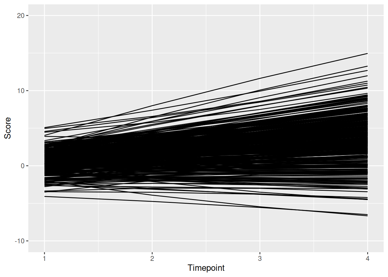
lavaanPlot::lavaanPlot(
  quadraticGCM1_fit,
  coefs = TRUE,
  #covs = TRUE,
stand = TRUE)lavaanPlot::lavaanPlot2(
quadraticGCM1_fit,
#stand = TRUE, # currently throws error; uncomment out when fixed: https://github.com/alishinski/lavaanPlot/issues/52
coef_labels = TRUE)To generate an interactive/modifiable path diagram, you can use the following syntax:
lavaangui::plot_lavaan(quadraticGCM1_fit)Calculated from intercept and slope parameters:
quadraticGCM1_intercept <- coef(quadraticGCM1_fit)["intercept~1"]
quadraticGCM1_linear <- coef(quadraticGCM1_fit)["linear~1"]
quadraticGCM1_quadratic <- coef(quadraticGCM1_fit)["quadratic~1"]

timepoints <- 4

newData <- data.frame(
  time = 1:4,
  linearLoading = c(0, 1, 2, 3),
  quadraticLoading = c(0, 1, 4, 9)
)

newData$predictedValue <- NA
newData$predictedValue <- quadraticGCM1_intercept + (quadraticGCM1_linear * newData$linearLoading) + (quadraticGCM1_quadratic * newData$quadraticLoading)

ggplot(
  data = newData,
  mapping = aes(
    x = time,
    y = predictedValue)) +
  geom_smooth(
    method = "lm",
    formula = y ~ x + I(x^2),
    se = FALSE,
    linewidth = 1
  ) +
  coord_cartesian(
    ylim = c(0, 5)) +
  labs(
    x = "Timepoint",
    y = "Score"
  ) +
  theme_classic()
person_factors <- as.data.frame(predict(quadraticGCM1_fit))
person_factors$id <- rownames(person_factors)

linear_loadings <- c(0, 1, 2, 3)
quadratic_loadings <- c(0, 1, 4, 9)

# Compute model-implied values for each person at each time point
individual_trajectories <- person_factors %>%
  rowwise() %>%
  mutate(
    t1 = intercept + (linear * linear_loadings[1]) + (quadratic * quadratic_loadings[1]),
    t2 = intercept + (linear * linear_loadings[2]) + (quadratic * quadratic_loadings[2]),
    t3 = intercept + (linear * linear_loadings[3]) + (quadratic * quadratic_loadings[3]),
    t4 = intercept + (linear * linear_loadings[4]) + (quadratic * quadratic_loadings[4])
  ) %>%
  ungroup() %>%
  select(id, t1, t2, t3, t4) %>%
  pivot_longer(
    cols = t1:t4,
    names_to = "timepoint",
    values_to = "value") %>%
  mutate(
    time = as.integer(substr(timepoint, 2, 2)) # extract number from "t1", "t2", etc.
  )

ggplot(
  data = individual_trajectories,
  mapping = aes(
    x = time,
    y = value,
    group = factor(id))) +
  geom_smooth(
    method = "lm",
    formula = y ~ x + I(x^2),
    se = FALSE,
    linewidth = 0.5
  ) +
  labs(
    x = "Timepoint",
    y = "Score"
  ) +
   theme_classic()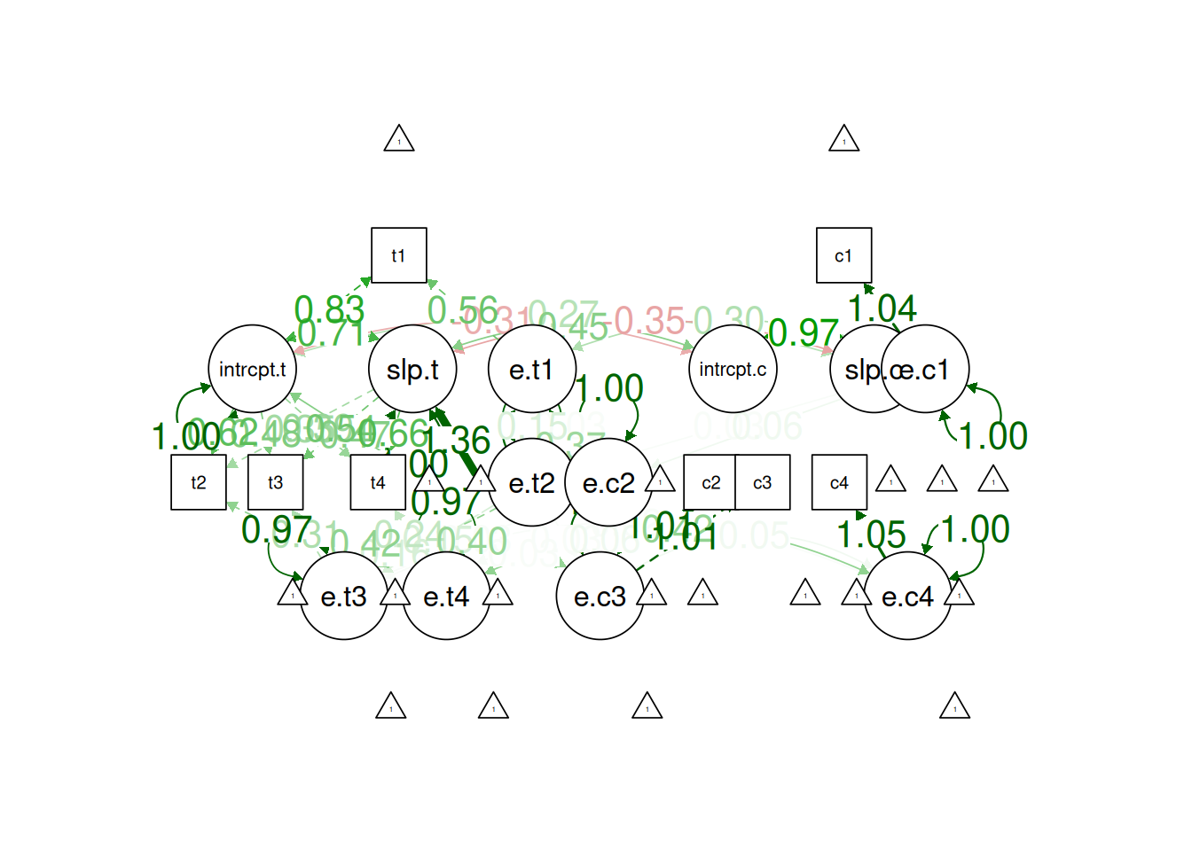
ggplot() +
  geom_smooth( # individuals' model-implied trajectories
    data = individual_trajectories,
    mapping = aes(
      x = time,
      y = value,
      group = id),
    method = "lm",
    formula = y ~ x + I(x^2),
    se = FALSE,
    linewidth = 0.5,
    color = "gray",
    alpha = 0.30
  ) +
  geom_smooth( # prototypical trajectory
    data = newData,
    mapping = aes(
      x = time,
      y = predictedValue),
    inherit.aes = FALSE,
    method = "lm",
    formula = y ~ x + I(x^2),
    se = FALSE,
    linewidth = 2
  ) +
  labs(
    x = "Timepoint",
    y = "Score"
  ) +
   theme_classic()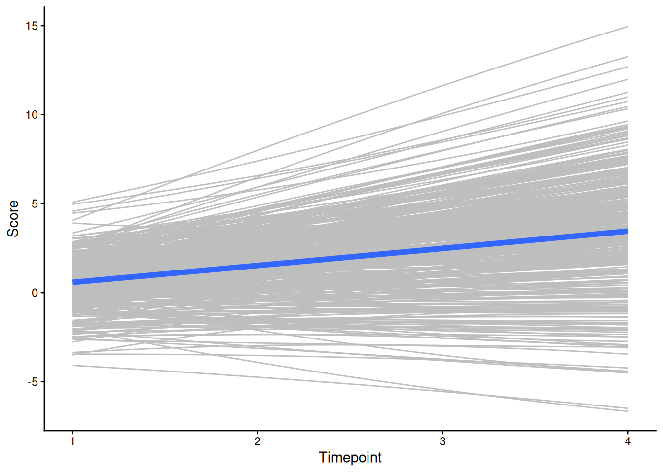
“an exponential pattern of change—in which change appears to ‘level off’ over time—can be approximated through linear (and potentially quadratic) slopes for a natural-log-transformed” version of time in a mixed-effects model or by fixing the latent change factor loadings to these values in SEM (Hoffman, 2025).
Can get the factor loadings via:
log(0:3 + 1)[1] 0.0000000 0.6931472 1.0986123 1.3862944logGCM1_syntax <- '
# Intercept and slope
intercept =~ 1*t1 + 1*t2 + 1*t3 + 1*t4
slope =~ 0*t1 + 0.6931472*t2 + 1.0986123*t3 + 1.3862944*t4
# Regression paths
intercept ~ x1 + x2
slope ~ x1 + x2
# Time-varying covariates
t1 ~ c1
t2 ~ c2
t3 ~ c3
t4 ~ c4
'logGCM2_syntax <- '
# Intercept and slope
intercept =~ 1*t1 + 1*t2 + 1*t3 + 1*t4
slope =~ 0*t1 + 0.6931472*t2 + 1.0986123*t3 + 1.3862944*t4
# Regression paths
intercept ~ x1 + x2
slope ~ x1 + x2
# Time-varying covariates
t1 ~ c1
t2 ~ c2
t3 ~ c3
t4 ~ c4
# Constrain observed intercepts to zero
t1 ~ 0*1
t2 ~ 0*1
t3 ~ 0*1
t4 ~ 0*1
# Estimate mean of intercept and slope
intercept ~ 1
slope ~ 1
'logGCM1_fit <- growth(
logGCM1_syntax,
data = Demo.growth,
missing = "ML",
estimator = "MLR",
meanstructure = TRUE,
int.ov.free = FALSE,
int.lv.free = TRUE,
fixed.x = FALSE,
em.h1.iter.max = 100000)logGCM2_fit <- sem(
logGCM2_syntax,
data = Demo.growth,
missing = "ML",
estimator = "MLR",
meanstructure = TRUE,
fixed.x = FALSE,
em.h1.iter.max = 100000)summary(
logGCM1_fit,
fit.measures = TRUE,
standardized = TRUE,
rsquare = TRUE)lavaan 0.6-21 ended normally after 31 iterations
Estimator ML
Optimization method NLMINB
Number of model parameters 38
Number of observations 400
Number of missing patterns 1
Model Test User Model:
Standard Scaled
Test Statistic 193.051 193.089
Degrees of freedom 27 27
P-value (Chi-square) 0.000 0.000
Scaling correction factor 1.000
Yuan-Bentler correction (Mplus variant)
Model Test Baseline Model:
Test statistic 2345.885 2414.540
Degrees of freedom 30 30
P-value 0.000 0.000
Scaling correction factor 0.972
User Model versus Baseline Model:
Comparative Fit Index (CFI) 0.928 0.930
Tucker-Lewis Index (TLI) 0.920 0.923
Robust Comparative Fit Index (CFI) 0.927
Robust Tucker-Lewis Index (TLI) 0.919
Loglikelihood and Information Criteria:
Loglikelihood user model (H0) -5858.646 -5858.646
Scaling correction factor 0.988
for the MLR correction
Loglikelihood unrestricted model (H1) -5762.120 -5762.120
Scaling correction factor 0.993
for the MLR correction
Akaike (AIC) 11793.291 11793.291
Bayesian (BIC) 11944.967 11944.967
Sample-size adjusted Bayesian (SABIC) 11824.391 11824.391
Root Mean Square Error of Approximation:
RMSEA 0.124 0.124
90 Percent confidence interval - lower 0.108 0.108
90 Percent confidence interval - upper 0.141 0.141
P-value H_0: RMSEA <= 0.050 0.000 0.000
P-value H_0: RMSEA >= 0.080 1.000 1.000
Robust RMSEA 0.124
90 Percent confidence interval - lower 0.108
90 Percent confidence interval - upper 0.141
P-value H_0: Robust RMSEA <= 0.050 0.000
P-value H_0: Robust RMSEA >= 0.080 1.000
Standardized Root Mean Square Residual:
SRMR 0.048 0.048
Parameter Estimates:
Standard errors Sandwich
Information bread Observed
Observed information based on Hessian
Latent Variables:
Estimate Std.Err z-value P(>|z|) Std.lv Std.all
intercept =~
t1 1.000 1.341 0.873
t2 1.000 1.341 0.591
t3 1.000 1.341 0.487
t4 1.000 1.341 0.418
slope =~
t1 0.000 0.000 0.000
t2 0.693 1.062 0.468
t3 1.099 1.683 0.611
t4 1.386 2.124 0.662
Regressions:
Estimate Std.Err z-value P(>|z|) Std.lv Std.all
intercept ~
x1 0.581 0.061 9.584 0.000 0.433 0.447
x2 0.535 0.065 8.228 0.000 0.399 0.387
slope ~
x1 0.511 0.059 8.703 0.000 0.334 0.344
x2 1.047 0.069 15.087 0.000 0.683 0.664
t1 ~
c1 0.138 0.047 2.947 0.003 0.138 0.089
t2 ~
c2 0.280 0.051 5.477 0.000 0.280 0.117
t3 ~
c3 0.312 0.051 6.169 0.000 0.312 0.106
t4 ~
c4 0.286 0.064 4.478 0.000 0.286 0.082
Covariances:
Estimate Std.Err z-value P(>|z|) Std.lv Std.all
.intercept ~~
.slope 0.076 0.118 0.641 0.521 0.078 0.078
x1 ~~
x2 0.141 0.050 2.798 0.005 0.141 0.140
c1 -0.039 0.051 -0.762 0.446 -0.039 -0.038
c2 0.023 0.048 0.493 0.622 0.023 0.024
c3 0.027 0.050 0.544 0.586 0.027 0.028
c4 -0.023 0.045 -0.519 0.604 -0.023 -0.024
x2 ~~
c1 -0.018 0.050 -0.358 0.721 -0.018 -0.019
c2 -0.003 0.044 -0.075 0.940 -0.003 -0.004
c3 0.155 0.048 3.239 0.001 0.155 0.170
c4 -0.104 0.043 -2.421 0.015 -0.104 -0.116
c1 ~~
c2 0.080 0.045 1.793 0.073 0.080 0.086
c3 -0.030 0.050 -0.585 0.559 -0.030 -0.032
c4 0.127 0.048 2.668 0.008 0.127 0.140
c2 ~~
c3 0.003 0.041 0.078 0.938 0.003 0.004
c4 0.031 0.044 0.715 0.475 0.031 0.036
c3 ~~
c4 0.034 0.044 0.767 0.443 0.034 0.039
Intercepts:
Estimate Std.Err z-value P(>|z|) Std.lv Std.all
.intercept 0.465 0.068 6.791 0.000 0.347 0.347
.slope 1.892 0.070 26.990 0.000 1.235 1.235
Variances:
Estimate Std.Err z-value P(>|z|) Std.lv Std.all
.t1 0.550 0.141 3.898 0.000 0.550 0.233
.t2 0.694 0.060 11.634 0.000 0.694 0.135
.t3 0.387 0.055 7.036 0.000 0.387 0.051
.t4 1.152 0.113 10.193 0.000 1.152 0.112
.intercept 1.082 0.148 7.295 0.000 0.602 0.602
.slope 0.885 0.133 6.664 0.000 0.377 0.377
x1 1.064 0.068 15.614 0.000 1.064 1.000
x2 0.943 0.065 14.401 0.000 0.943 1.000
c1 0.972 0.064 15.306 0.000 0.972 1.000
c2 0.900 0.063 14.372 0.000 0.900 1.000
c3 0.876 0.067 13.041 0.000 0.876 1.000
c4 0.852 0.057 15.005 0.000 0.852 1.000
R-Square:
Estimate
t1 0.767
t2 0.865
t3 0.949
t4 0.888
intercept 0.398
slope 0.623summary(
logGCM2_fit,
fit.measures = TRUE,
standardized = TRUE,
rsquare = TRUE)lavaan 0.6-21 ended normally after 31 iterations
Estimator ML
Optimization method NLMINB
Number of model parameters 44
Number of observations 400
Number of missing patterns 1
Model Test User Model:
Standard Scaled
Test Statistic 178.336 179.152
Degrees of freedom 21 21
P-value (Chi-square) 0.000 0.000
Scaling correction factor 0.995
Yuan-Bentler correction (Mplus variant)
Model Test Baseline Model:
Test statistic 2345.885 2414.540
Degrees of freedom 30 30
P-value 0.000 0.000
Scaling correction factor 0.972
User Model versus Baseline Model:
Comparative Fit Index (CFI) 0.932 0.934
Tucker-Lewis Index (TLI) 0.903 0.905
Robust Comparative Fit Index (CFI) 0.933
Robust Tucker-Lewis Index (TLI) 0.904
Loglikelihood and Information Criteria:
Loglikelihood user model (H0) -5851.288 -5851.288
Scaling correction factor 0.991
for the MLR correction
Loglikelihood unrestricted model (H1) -5762.120 -5762.120
Scaling correction factor 0.993
for the MLR correction
Akaike (AIC) 11790.576 11790.576
Bayesian (BIC) 11966.200 11966.200
Sample-size adjusted Bayesian (SABIC) 11826.585 11826.585
Root Mean Square Error of Approximation:
RMSEA 0.137 0.137
90 Percent confidence interval - lower 0.119 0.119
90 Percent confidence interval - upper 0.156 0.156
P-value H_0: RMSEA <= 0.050 0.000 0.000
P-value H_0: RMSEA >= 0.080 1.000 1.000
Robust RMSEA 0.135
90 Percent confidence interval - lower 0.116
90 Percent confidence interval - upper 0.156
P-value H_0: Robust RMSEA <= 0.050 0.000
P-value H_0: Robust RMSEA >= 0.080 1.000
Standardized Root Mean Square Residual:
SRMR 0.041 0.041
Parameter Estimates:
Standard errors Sandwich
Information bread Observed
Observed information based on Hessian
Latent Variables:
Estimate Std.Err z-value P(>|z|) Std.lv Std.all
intercept =~
t1 1.000 1.341 0.873
t2 1.000 1.341 0.592
t3 1.000 1.341 0.488
t4 1.000 1.341 0.418
slope =~
t1 0.000 0.000 0.000
t2 0.693 1.060 0.468
t3 1.099 1.680 0.611
t4 1.386 2.119 0.662
Regressions:
Estimate Std.Err z-value P(>|z|) Std.lv Std.all
intercept ~
x1 0.581 0.061 9.584 0.000 0.433 0.445
x2 0.535 0.065 8.228 0.000 0.399 0.383
slope ~
x1 0.511 0.059 8.703 0.000 0.334 0.343
x2 1.047 0.069 15.087 0.000 0.685 0.658
t1 ~
c1 0.138 0.047 2.947 0.003 0.138 0.089
t2 ~
c2 0.280 0.051 5.477 0.000 0.280 0.117
t3 ~
c3 0.312 0.051 6.169 0.000 0.312 0.106
t4 ~
c4 0.286 0.064 4.478 0.000 0.286 0.082
Covariances:
Estimate Std.Err z-value P(>|z|) Std.lv Std.all
.intercept ~~
.slope 0.076 0.118 0.641 0.521 0.078 0.078
x1 ~~
x2 0.153 0.049 3.129 0.002 0.153 0.155
c1 -0.038 0.050 -0.760 0.447 -0.038 -0.037
c2 0.026 0.048 0.547 0.585 0.026 0.027
c3 0.033 0.049 0.674 0.501 0.033 0.035
c4 -0.025 0.044 -0.560 0.575 -0.025 -0.026
x2 ~~
c1 -0.019 0.050 -0.377 0.706 -0.019 -0.020
c2 -0.007 0.044 -0.167 0.867 -0.007 -0.008
c3 0.145 0.048 3.055 0.002 0.145 0.162
c4 -0.102 0.043 -2.371 0.018 -0.102 -0.115
c1 ~~
c2 0.080 0.045 1.789 0.074 0.080 0.085
c3 -0.030 0.050 -0.596 0.551 -0.030 -0.033
c4 0.128 0.048 2.669 0.008 0.128 0.140
c2 ~~
c3 0.001 0.042 0.030 0.976 0.001 0.001
c4 0.032 0.044 0.729 0.466 0.032 0.036
c3 ~~
c4 0.035 0.044 0.796 0.426 0.035 0.041
Intercepts:
Estimate Std.Err z-value P(>|z|) Std.lv Std.all
.t1 0.000 0.000 0.000
.t2 0.000 0.000 0.000
.t3 0.000 0.000 0.000
.t4 0.000 0.000 0.000
.intercept 0.465 0.068 6.791 0.000 0.347 0.347
.slope 1.892 0.070 26.990 0.000 1.238 1.238
x1 -0.092 0.051 -1.793 0.073 -0.092 -0.090
x2 0.138 0.048 2.878 0.004 0.138 0.144
c1 0.008 0.049 0.158 0.874 0.008 0.008
c2 0.029 0.047 0.610 0.542 0.029 0.031
c3 0.068 0.047 1.449 0.147 0.068 0.072
c4 -0.018 0.046 -0.390 0.696 -0.018 -0.020
Variances:
Estimate Std.Err z-value P(>|z|) Std.lv Std.all
.t1 0.550 0.141 3.898 0.000 0.550 0.233
.t2 0.694 0.060 11.634 0.000 0.694 0.135
.t3 0.387 0.055 7.036 0.000 0.387 0.051
.t4 1.152 0.113 10.193 0.000 1.152 0.112
.intercept 1.082 0.148 7.295 0.000 0.602 0.602
.slope 0.885 0.133 6.664 0.000 0.379 0.379
x1 1.056 0.068 15.511 0.000 1.056 1.000
x2 0.924 0.065 14.153 0.000 0.924 1.000
c1 0.972 0.063 15.321 0.000 0.972 1.000
c2 0.899 0.062 14.432 0.000 0.899 1.000
c3 0.872 0.067 13.018 0.000 0.872 1.000
c4 0.851 0.057 15.001 0.000 0.851 1.000
R-Square:
Estimate
t1 0.767
t2 0.865
t3 0.949
t4 0.888
intercept 0.398
slope 0.621fitMeasures(
logGCM1_fit,
fit.measures = c(
"chisq", "df", "pvalue",
"chisq.scaled", "df.scaled", "pvalue.scaled",
"chisq.scaling.factor",
"baseline.chisq","baseline.df","baseline.pvalue",
"rmsea", "cfi", "tli", "srmr",
"rmsea.robust", "cfi.robust", "tli.robust")) chisq df pvalue
193.051 27.000 0.000
chisq.scaled df.scaled pvalue.scaled
193.089 27.000 0.000
chisq.scaling.factor baseline.chisq baseline.df
1.000 2345.885 30.000
baseline.pvalue rmsea cfi
0.000 0.124 0.928
tli srmr rmsea.robust
0.920 0.048 0.124
cfi.robust tli.robust
0.927 0.919 residuals(
logGCM1_fit,
type = "cor")$type
[1] "cor.bollen"
$cov
t1 t2 t3 t4 x1 x2 c1 c2 c3 c4
t1 0.000
t2 0.046 0.000
t3 0.016 -0.016 0.000
t4 0.054 0.012 0.024 0.000
x1 0.017 0.004 0.000 0.025 0.000
x2 0.027 -0.014 -0.006 0.022 0.015 0.000
c1 0.005 0.019 0.001 0.056 0.001 -0.001 0.000
c2 0.006 0.008 -0.007 -0.005 0.003 -0.004 0.000 0.000
c3 0.051 0.015 0.034 0.035 0.007 -0.008 -0.001 -0.002 0.000
c4 0.034 0.029 0.002 0.011 -0.002 0.002 0.000 0.001 0.002 0.000
$mean
t1 t2 t3 t4 x1 x2 c1 c2 c3 c4
0.082 -0.049 0.018 0.163 -0.090 0.144 0.008 0.031 0.072 -0.020 modificationindices(
logGCM1_fit,
sort. = TRUE)compRelSEM(logGCM1_fit)Error in `PHI[[b.idx]][myFacNames, myFacNames, drop = FALSE]`:
! subscript out of boundssemPlot::semPaths(
logGCM1_fit,
what = "Std.all",
layout = "tree2",
edge.label.cex = 1.5)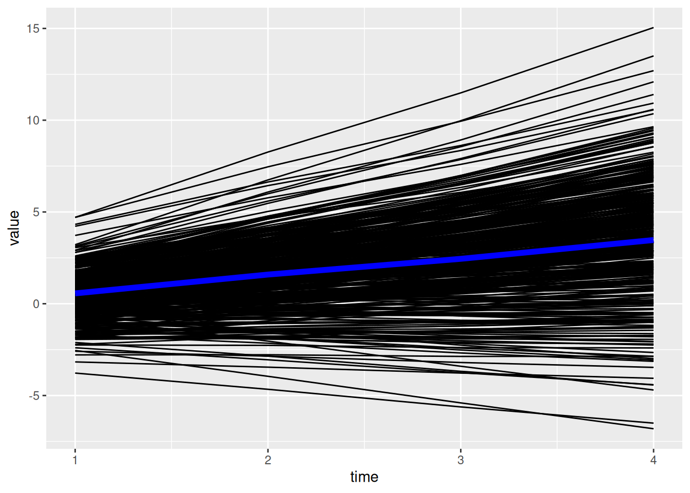
lavaanPlot::lavaanPlot(
  logGCM1_fit,
  coefs = TRUE,
  #covs = TRUE,
stand = TRUE)lavaanPlot::lavaanPlot2(
logGCM1_fit,
#stand = TRUE, # currently throws error; uncomment out when fixed: https://github.com/alishinski/lavaanPlot/issues/52
coef_labels = TRUE)To generate an interactive/modifiable path diagram, you can use the following syntax:
lavaangui::plot_lavaan(logGCM1_fit)logGCM1_intercept <- coef(logGCM1_fit)["intercept~1"]
logGCM1_slope <- coef(logGCM1_fit)["slope~1"]
timepoints <- 4
newData <- data.frame(
time = c(1, 4),
logLoading = c(0, 0.6931472, 1.0986123, 1.3862944)
)
newData$predictedValue <- NA
newData$predictedValue <- logGCM1_intercept + (logGCM1_slope * newData$logLoading)
ggplot(
data = newData,
mapping = aes(
x = time,
y = predictedValue)) +
geom_line(
stat = "smooth",
method = "lm",
formula = y ~ log(x + 1),
se = FALSE,
linewidth = 1,
) +
coord_cartesian(
ylim = c(0, 5)) +
labs(
x = "Timepoint",
y = "Score"
) +
theme_classic()
person_factors <- as.data.frame(predict(logGCM1_fit))
person_factors$id <- rownames(person_factors)

linear_loadings <- c(0, 1, 2, 3)
log_loadings <- c(0, 0.6931472, 1.0986123, 1.3862944)

# Compute model-implied values for each person at each time point
individual_trajectories <- person_factors %>%
  rowwise() %>%
  mutate(
    t1 = intercept + (slope * log_loadings[1]),
    t2 = intercept + (slope * log_loadings[2]),
    t3 = intercept + (slope * log_loadings[3]),
    t4 = intercept + (slope * log_loadings[4])
  ) %>%
  ungroup() %>%
  select(id, t1, t2, t3, t4) %>%
  pivot_longer(
    cols = t1:t4,
    names_to = "timepoint",
    values_to = "value") %>%
  mutate(
    time = as.integer(substr(timepoint, 2, 2)) # extract number from "t1", "t2", etc.
  )

ggplot(
  data = individual_trajectories,
  mapping = aes(
    x = time,
    y = value,
    group = factor(id))) +
  geom_smooth(
    method = "lm",
    formula = y ~ log(x + 1),
    se = FALSE,
    linewidth = 0.5
  ) +
  labs(
    x = "Timepoint",
    y = "Score"
  ) +
   theme_classic()
ggplot() +
  geom_smooth( # individuals' model-implied trajectories
    data = individual_trajectories,
    mapping = aes(
      x = time,
      y = value,
      group = id),
    method = "lm",
    formula = y ~ log(x + 1),
    se = FALSE,
    linewidth = 0.5,
    color = "gray",
    alpha = 0.30
  ) +
  geom_smooth( # prototypical trajectory
    data = newData,
    mapping = aes(
      x = time,
      y = predictedValue),
    method = "lm",
    formula = y ~ log(x + 1),
    se = FALSE,
    linewidth = 2
  ) +
  labs(
    x = "Timepoint",
    y = "Score"
  ) +
   theme_classic()
splineGCM1_syntax <- '
  # Intercept and slope
  intercept =~ 1*t1 + 1*t2 + 1*t3 + 1*t4
  slope =~ 0*t1 + 1*t2 + 2*t3 + 3*t4
  knot =~ 0*t1 + 0*t2 + 1*t3 + 1*t4

  # Regression paths
  intercept ~ x1 + x2
  slope ~ x1 + x2
  knot ~ x1 + x2

  # Spline has no variance
  knot ~~ 0*knot

  # Spline does not covary with intercept and slope
  knot ~~ 0*intercept
  knot ~~ 0*slope

  # Time-varying covariates
  t1 ~ c1
  t2 ~ c2
  t3 ~ c3
  t4 ~ c4
'splineGCM2_syntax <- '
# Intercept and slope
intercept =~ 1*t1 + 1*t2 + 1*t3 + 1*t4
slope =~ 0*t1 + 1*t2 + 2*t3 + 3*t4
knot =~ 0*t1 + 0*t2 + 1*t3 + 1*t4
# Regression paths
intercept ~ x1 + x2
slope ~ x1 + x2
knot ~ x1 + x2
# Spline has no variance
knot ~~ 0*knot
# Spline does not covary with intercept and slope
knot ~~ 0*intercept
knot ~~ 0*slope
# Time-varying covariates
t1 ~ c1
t2 ~ c2
t3 ~ c3
t4 ~ c4
# Constrain observed intercepts to zero
t1 ~ 0*1
t2 ~ 0*1
t3 ~ 0*1
t4 ~ 0*1
# Estimate mean of intercept and slope
intercept ~ 1
slope ~ 1
knot ~ 1
'splineGCM1_fit <- growth(
splineGCM1_syntax,
data = Demo.growth,
missing = "ML",
estimator = "MLR",
meanstructure = TRUE,
int.ov.free = FALSE,
int.lv.free = TRUE,
fixed.x = FALSE,
em.h1.iter.max = 100000)splineGCM2_fit <- sem(
splineGCM2_syntax,
data = Demo.growth,
missing = "ML",
estimator = "MLR",
meanstructure = TRUE,
fixed.x = FALSE,
em.h1.iter.max = 100000)summary(
splineGCM1_fit,
fit.measures = TRUE,
standardized = TRUE,
rsquare = TRUE)lavaan 0.6-21 ended normally after 35 iterations
Estimator ML
Optimization method NLMINB
Number of model parameters 41
Number of observations 400
Number of missing patterns 1
Model Test User Model:
Standard Scaled
Test Statistic 36.091 36.117
Degrees of freedom 24 24
P-value (Chi-square) 0.054 0.053
Scaling correction factor 0.999
Yuan-Bentler correction (Mplus variant)
Model Test Baseline Model:
Test statistic 2345.885 2414.540
Degrees of freedom 30 30
P-value 0.000 0.000
Scaling correction factor 0.972
User Model versus Baseline Model:
Comparative Fit Index (CFI) 0.995 0.995
Tucker-Lewis Index (TLI) 0.993 0.994
Robust Comparative Fit Index (CFI) 0.993
Robust Tucker-Lewis Index (TLI) 0.991
Loglikelihood and Information Criteria:
Loglikelihood user model (H0) -5780.166 -5780.166
Scaling correction factor 0.989
for the MLR correction
Loglikelihood unrestricted model (H1) -5762.120 -5762.120
Scaling correction factor 0.993
for the MLR correction
Akaike (AIC) 11642.331 11642.331
Bayesian (BIC) 11805.981 11805.981
Sample-size adjusted Bayesian (SABIC) 11675.885 11675.885
Root Mean Square Error of Approximation:
RMSEA 0.035 0.036
90 Percent confidence interval - lower 0.000 0.000
90 Percent confidence interval - upper 0.058 0.058
P-value H_0: RMSEA <= 0.050 0.841 0.840
P-value H_0: RMSEA >= 0.080 0.000 0.000
Robust RMSEA 0.041
90 Percent confidence interval - lower 0.019
90 Percent confidence interval - upper 0.060
P-value H_0: Robust RMSEA <= 0.050 0.768
P-value H_0: Robust RMSEA >= 0.080 0.000
Standardized Root Mean Square Residual:
SRMR 0.029 0.029
Parameter Estimates:
Standard errors Sandwich
Information bread Observed
Observed information based on Hessian
Latent Variables:
Estimate Std.Err z-value P(>|z|) Std.lv Std.all
intercept =~
t1 1.000 1.383 0.874
t2 1.000 1.383 0.655
t3 1.000 1.383 0.508
t4 1.000 1.383 0.410
slope =~
t1 0.000 0.000 0.000
t2 1.000 0.787 0.373
t3 2.000 1.573 0.578
t4 3.000 2.360 0.699
knot =~
t1 0.000 0.000 0.000
t2 0.000 0.000 0.000
t3 1.000 0.059 0.022
t4 1.000 0.059 0.017
Regressions:
Estimate Std.Err z-value P(>|z|) Std.lv Std.all
intercept ~
x1 0.604 0.059 10.254 0.000 0.437 0.451
x2 0.601 0.061 9.824 0.000 0.435 0.422
slope ~
x1 0.280 0.042 6.705 0.000 0.356 0.367
x2 0.535 0.043 12.349 0.000 0.680 0.660
knot ~
x1 -0.044 0.077 -0.572 0.568 -0.746 -0.770
x2 -0.033 0.088 -0.372 0.710 -0.555 -0.539
t1 ~
c1 0.143 0.045 3.194 0.001 0.143 0.089
t2 ~
c2 0.287 0.047 6.129 0.000 0.287 0.129
t3 ~
c3 0.336 0.047 7.074 0.000 0.336 0.115
t4 ~
c4 0.333 0.057 5.871 0.000 0.333 0.091
Covariances:
Estimate Std.Err z-value P(>|z|) Std.lv Std.all
.intercept ~~
.knot 0.000 NaN NaN
.slope ~~
.knot 0.000 NaN NaN
.intercept ~~
.slope 0.075 0.039 1.892 0.059 0.152 0.152
x1 ~~
x2 0.141 0.050 2.798 0.005 0.141 0.140
c1 -0.039 0.051 -0.762 0.446 -0.039 -0.038
c2 0.023 0.048 0.493 0.622 0.023 0.024
c3 0.027 0.050 0.544 0.586 0.027 0.028
c4 -0.023 0.045 -0.519 0.604 -0.023 -0.024
x2 ~~
c1 -0.018 0.050 -0.358 0.721 -0.018 -0.019
c2 -0.003 0.044 -0.075 0.940 -0.003 -0.004
c3 0.155 0.048 3.239 0.001 0.155 0.170
c4 -0.104 0.043 -2.421 0.015 -0.104 -0.116
c1 ~~
c2 0.080 0.045 1.793 0.073 0.080 0.086
c3 -0.030 0.050 -0.585 0.559 -0.030 -0.032
c4 0.127 0.048 2.668 0.008 0.127 0.140
c2 ~~
c3 0.003 0.041 0.078 0.938 0.003 0.004
c4 0.031 0.044 0.715 0.475 0.031 0.036
c3 ~~
c4 0.034 0.044 0.767 0.443 0.034 0.039
Intercepts:
Estimate Std.Err z-value P(>|z|) Std.lv Std.all
.intercept 0.565 0.061 9.265 0.000 0.409 0.409
.slope 1.025 0.042 24.178 0.000 1.303 1.303
.knot -0.167 0.081 -2.058 0.040 -2.839 -2.839
Variances:
Estimate Std.Err z-value P(>|z|) Std.lv Std.all
.knot 0.000 0.000 0.000
.t1 0.581 0.091 6.403 0.000 0.581 0.232
.t2 0.591 0.055 10.763 0.000 0.591 0.133
.t3 0.475 0.051 9.390 0.000 0.475 0.064
.t4 0.538 0.093 5.768 0.000 0.538 0.047
.intercept 1.080 0.108 10.010 0.000 0.565 0.565
.slope 0.224 0.027 8.392 0.000 0.361 0.361
x1 1.064 0.068 15.614 0.000 1.064 1.000
x2 0.943 0.065 14.401 0.000 0.943 1.000
c1 0.972 0.064 15.306 0.000 0.972 1.000
c2 0.900 0.063 14.372 0.000 0.900 1.000
c3 0.876 0.067 13.041 0.000 0.876 1.000
c4 0.852 0.057 15.005 0.000 0.852 1.000
R-Square:
Estimate
knot 1.000
t1 0.768
t2 0.867
t3 0.936
t4 0.953
intercept 0.435
slope 0.639summary(
splineGCM2_fit,
fit.measures = TRUE,
standardized = TRUE,
rsquare = TRUE)lavaan 0.6-21 ended normally after 39 iterations
Estimator ML
Optimization method NLMINB
Number of model parameters 47
Number of observations 400
Number of missing patterns 1
Model Test User Model:
Standard Scaled
Test Statistic 21.375 21.504
Degrees of freedom 18 18
P-value (Chi-square) 0.261 0.255
Scaling correction factor 0.994
Yuan-Bentler correction (Mplus variant)
Model Test Baseline Model:
Test statistic 2345.885 2414.540
Degrees of freedom 30 30
P-value 0.000 0.000
Scaling correction factor 0.972
User Model versus Baseline Model:
Comparative Fit Index (CFI) 0.999 0.999
Tucker-Lewis Index (TLI) 0.998 0.998
Robust Comparative Fit Index (CFI) 0.999
Robust Tucker-Lewis Index (TLI) 0.998
Loglikelihood and Information Criteria:
Loglikelihood user model (H0) -5772.808 -5772.808
Scaling correction factor 0.992
for the MLR correction
Loglikelihood unrestricted model (H1) -5762.120 -5762.120
Scaling correction factor 0.993
for the MLR correction
Akaike (AIC) 11639.615 11639.615
Bayesian (BIC) 11827.214 11827.214
Sample-size adjusted Bayesian (SABIC) 11678.080 11678.080
Root Mean Square Error of Approximation:
RMSEA 0.022 0.022
90 Percent confidence interval - lower 0.000 0.000
90 Percent confidence interval - upper 0.052 0.052
P-value H_0: RMSEA <= 0.050 0.938 0.935
P-value H_0: RMSEA >= 0.080 0.000 0.000
Robust RMSEA 0.022
90 Percent confidence interval - lower 0.000
90 Percent confidence interval - upper 0.052
P-value H_0: Robust RMSEA <= 0.050 0.938
P-value H_0: Robust RMSEA >= 0.080 0.000
Standardized Root Mean Square Residual:
SRMR 0.013 0.013
Parameter Estimates:
Standard errors Sandwich
Information bread Observed
Observed information based on Hessian
Latent Variables:
Estimate Std.Err z-value P(>|z|) Std.lv Std.all
intercept =~
t1 1.000 1.382 0.874
t2 1.000 1.382 0.655
t3 1.000 1.382 0.508
t4 1.000 1.382 0.410
slope =~
t1 0.000 0.000 0.000
t2 1.000 0.785 0.372
t3 2.000 1.570 0.577
t4 3.000 2.355 0.699
knot =~
t1 0.000 0.000 0.000
t2 0.000 0.000 0.000
t3 1.000 0.059 0.022
t4 1.000 0.059 0.017
Regressions:
Estimate Std.Err z-value P(>|z|) Std.lv Std.all
intercept ~
x1 0.604 0.059 10.254 0.000 0.437 0.449
x2 0.601 0.061 9.824 0.000 0.435 0.418
slope ~
x1 0.280 0.042 6.705 0.000 0.356 0.366
x2 0.535 0.043 12.349 0.000 0.681 0.655
knot ~
x1 -0.044 0.077 -0.572 0.568 -0.746 -0.767
x2 -0.033 0.088 -0.372 0.710 -0.555 -0.534
t1 ~
c1 0.143 0.045 3.194 0.001 0.143 0.089
t2 ~
c2 0.287 0.047 6.129 0.000 0.287 0.129
t3 ~
c3 0.336 0.047 7.074 0.000 0.336 0.115
t4 ~
c4 0.333 0.057 5.871 0.000 0.333 0.091
Covariances:
Estimate Std.Err z-value P(>|z|) Std.lv Std.all
.intercept ~~
.knot 0.000 NaN NaN
.slope ~~
.knot 0.000 NaN NaN
.intercept ~~
.slope 0.075 0.039 1.892 0.059 0.152 0.152
x1 ~~
x2 0.153 0.049 3.129 0.002 0.153 0.155
c1 -0.038 0.050 -0.760 0.447 -0.038 -0.037
c2 0.026 0.048 0.547 0.585 0.026 0.027
c3 0.033 0.049 0.674 0.501 0.033 0.035
c4 -0.025 0.044 -0.560 0.575 -0.025 -0.026
x2 ~~
c1 -0.019 0.050 -0.377 0.706 -0.019 -0.020
c2 -0.007 0.044 -0.167 0.867 -0.007 -0.008
c3 0.145 0.048 3.055 0.002 0.145 0.162
c4 -0.102 0.043 -2.371 0.018 -0.102 -0.115
c1 ~~
c2 0.080 0.045 1.789 0.074 0.080 0.085
c3 -0.030 0.050 -0.596 0.551 -0.030 -0.033
c4 0.128 0.048 2.669 0.008 0.128 0.140
c2 ~~
c3 0.001 0.042 0.030 0.976 0.001 0.001
c4 0.032 0.044 0.729 0.466 0.032 0.036
c3 ~~
c4 0.035 0.044 0.796 0.426 0.035 0.041
Intercepts:
Estimate Std.Err z-value P(>|z|) Std.lv Std.all
.t1 0.000 0.000 0.000
.t2 0.000 0.000 0.000
.t3 0.000 0.000 0.000
.t4 0.000 0.000 0.000
.intercept 0.565 0.061 9.265 0.000 0.409 0.409
.slope 1.025 0.042 24.178 0.000 1.305 1.305
.knot -0.167 0.081 -2.058 0.040 -2.839 -2.839
x1 -0.092 0.051 -1.793 0.073 -0.092 -0.090
x2 0.138 0.048 2.878 0.004 0.138 0.144
c1 0.008 0.049 0.158 0.874 0.008 0.008
c2 0.029 0.047 0.610 0.542 0.029 0.031
c3 0.068 0.047 1.449 0.147 0.068 0.072
c4 -0.018 0.046 -0.390 0.696 -0.018 -0.020
Variances:
Estimate Std.Err z-value P(>|z|) Std.lv Std.all
.knot 0.000 0.000 0.000
.t1 0.581 0.091 6.403 0.000 0.581 0.232
.t2 0.591 0.055 10.763 0.000 0.591 0.133
.t3 0.475 0.051 9.390 0.000 0.475 0.064
.t4 0.538 0.093 5.768 0.000 0.538 0.047
.intercept 1.080 0.108 10.010 0.000 0.565 0.565
.slope 0.224 0.027 8.392 0.000 0.363 0.363
x1 1.056 0.068 15.511 0.000 1.056 1.000
x2 0.924 0.065 14.153 0.000 0.924 1.000
c1 0.972 0.063 15.321 0.000 0.972 1.000
c2 0.899 0.062 14.432 0.000 0.899 1.000
c3 0.872 0.067 13.018 0.000 0.872 1.000
c4 0.851 0.057 15.001 0.000 0.851 1.000
R-Square:
Estimate
knot 1.000
t1 0.768
t2 0.867
t3 0.936
t4 0.953
intercept 0.435
slope 0.637fitMeasures(
splineGCM1_fit,
fit.measures = c(
"chisq", "df", "pvalue",
"chisq.scaled", "df.scaled", "pvalue.scaled",
"chisq.scaling.factor",
"baseline.chisq","baseline.df","baseline.pvalue",
"rmsea", "cfi", "tli", "srmr",
"rmsea.robust", "cfi.robust", "tli.robust")) chisq df pvalue
36.091 24.000 0.054
chisq.scaled df.scaled pvalue.scaled
36.117 24.000 0.053
chisq.scaling.factor baseline.chisq baseline.df
0.999 2345.885 30.000
baseline.pvalue rmsea cfi
0.000 0.035 0.995
tli srmr rmsea.robust
0.993 0.029 0.041
cfi.robust tli.robust
0.993 0.991 residuals(
splineGCM1_fit,
type = "cor")$type
[1] "cor.bollen"
$cov
t1 t2 t3 t4 x1 x2 c1 c2 c3 c4
t1 0.000
t2 0.010 0.000
t3 -0.011 -0.002 0.000
t4 0.014 0.000 0.002 0.000
x1 0.009 -0.001 0.005 0.009 0.000
x2 -0.004 0.002 0.003 -0.003 0.015 0.000
c1 0.005 0.018 0.001 0.056 0.001 -0.001 0.000
c2 0.006 -0.004 -0.007 -0.005 0.003 -0.004 0.000 0.000
c3 0.046 0.018 0.027 0.030 0.007 -0.008 -0.001 -0.002 0.000
c4 0.038 0.027 0.001 0.005 -0.002 0.002 0.000 0.001 0.002 0.000
$mean
t1 t2 t3 t4 x1 x2 c1 c2 c3 c4
0.019 0.039 0.053 0.049 -0.090 0.144 0.008 0.031 0.072 -0.020 modificationindices(
splineGCM1_fit,
sort. = TRUE)compRelSEM(splineGCM1_fit)Error in `PHI[[b.idx]][myFacNames, myFacNames, drop = FALSE]`:
! subscript out of boundssemPlot::semPaths(
splineGCM1_fit,
what = "Std.all",
layout = "tree2",
edge.label.cex = 1.5)
lavaanPlot::lavaanPlot(
  splineGCM1_fit,
  coefs = TRUE,
  #covs = TRUE,
stand = TRUE)lavaanPlot::lavaanPlot2(
splineGCM1_fit,
#stand = TRUE, # currently throws error; uncomment out when fixed: https://github.com/alishinski/lavaanPlot/issues/52
coef_labels = TRUE)To generate an interactive/modifiable path diagram, you can use the following syntax:
lavaangui::plot_lavaan(splineGCM1_fit)Calculated from intercept and slope parameters:
splineGCM1_intercept <- coef(splineGCM1_fit)["intercept~1"]
splineGCM1_slope <- coef(splineGCM1_fit)["slope~1"]
splineGCM1_knot <- coef(splineGCM1_fit)["knot~1"]

timepoints <- 4

newData <- data.frame(
  time = 1:4,
  linearLoading = c(0, 1, 2, 3),
  knotLoading = c(0, 0, 1, 1)
)

newData$predictedValue <- NA
newData$predictedValue <- splineGCM1_intercept + (splineGCM1_slope * newData$linearLoading) + (splineGCM1_knot * newData$knotLoading)

ggplot(
  data = newData,
  mapping = aes(
    x = time,
    y = predictedValue)) +
  geom_line(
    linewidth = 1
  ) +
  coord_cartesian(
    ylim = c(0, 5)) +
  labs(
    x = "Timepoint",
    y = "Score"
  ) +
  theme_classic()
person_factors <- as.data.frame(predict(splineGCM1_fit))
person_factors$id <- rownames(person_factors)

slope_loadings <- c(0, 1, 2, 3)
knot_loadings <- c(0, 0, 1, 1)

# Compute model-implied values for each person at each time point
individual_trajectories <- person_factors %>%
  rowwise() %>%
  mutate(
    t1 = intercept + (slope * slope_loadings[1]) + (knot * knot_loadings[1]),
    t2 = intercept + (slope * slope_loadings[2]) + (knot * knot_loadings[2]),
    t3 = intercept + (slope * slope_loadings[3]) + (knot * knot_loadings[3]),
    t4 = intercept + (slope * slope_loadings[4]) + (knot * knot_loadings[4])
  ) %>%
  ungroup() %>%
  select(id, t1, t2, t3, t4) %>%
  pivot_longer(
    cols = t1:t4,
    names_to = "timepoint",
    values_to = "value") %>%
  mutate(
    time = as.integer(substr(timepoint, 2, 2)) # extract number from "t1", "t2", etc.
  )

ggplot(
  data = individual_trajectories,
  mapping = aes(
    x = time,
    y = value,
    group = factor(id))) +
  geom_line() +
  labs(
    x = "Timepoint",
    y = "Score"
  ) +
   theme_classic()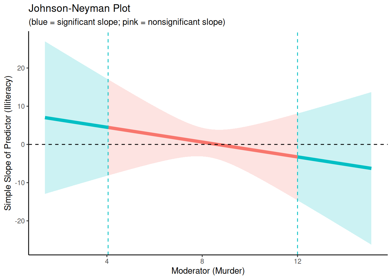
ggplot() +
  geom_line( # individuals' model-implied trajectories
    data = individual_trajectories,
    aes(
      x = time,
      y = value,
      group = id),
    linewidth = 0.5,
    color = "gray",
    alpha = 0.30
  ) +
  geom_line( # prototypical trajectory
    data = newData,
    aes(
      x = time,
      y = predictedValue),
    color = "blue",
    linewidth = 2
  ) +
  labs(
    x = "Timepoint",
    y = "Score"
  ) +
   theme_classic()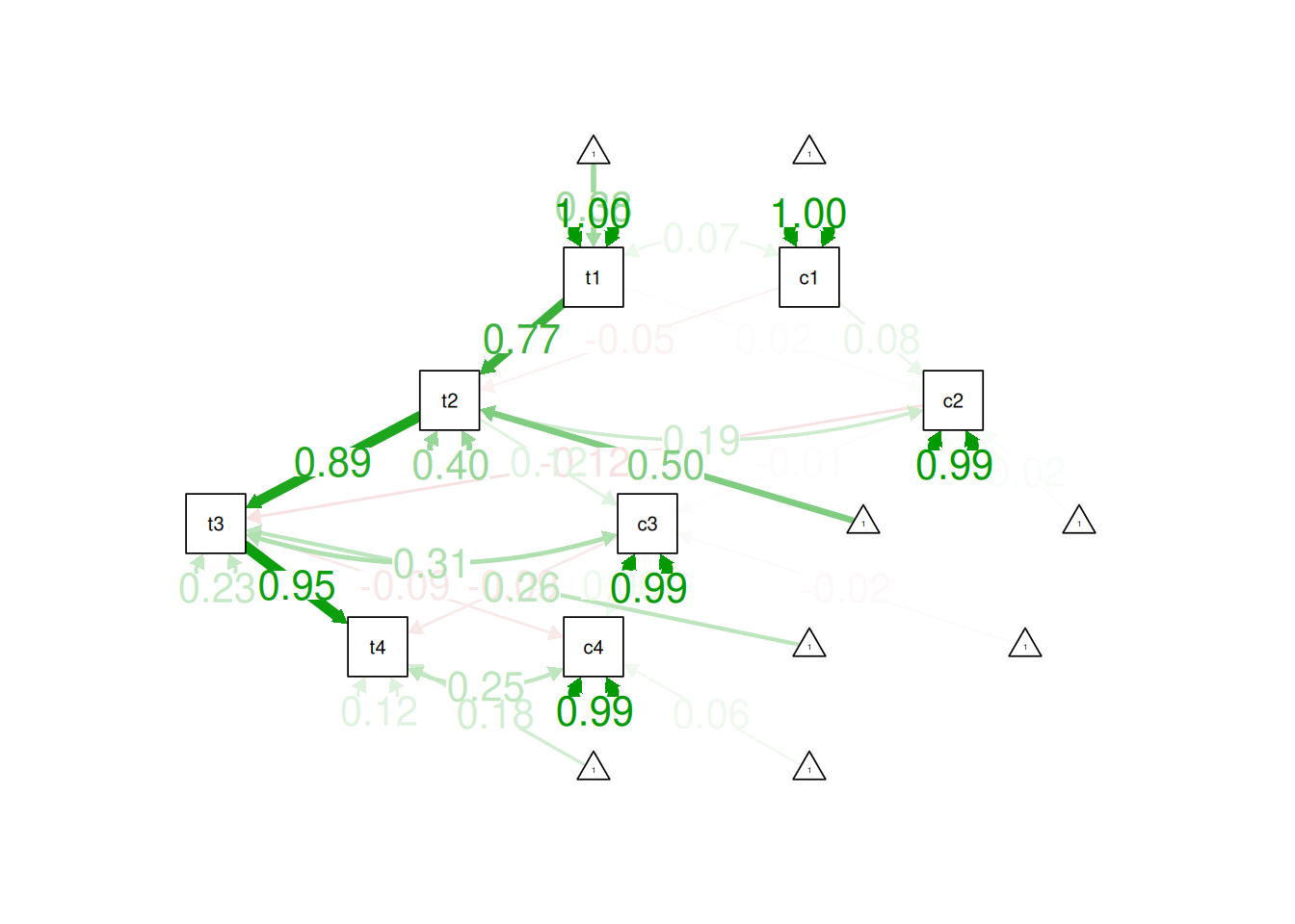
https://tdjorgensen.github.io/SEM-in-Ed-compendium/ch27.html#saturated-growth-model (archived at https://perma.cc/2CJX-WLLZ)
An example of a second-order latent growth curve model is here.
To generate the syntax for a latent change score model, we use the lcsm package.
bivariateLCSM_syntax <- lcsm::specify_bi_lcsm(
  timepoints = 3,
  var_x = "x",
  model_x = list(
    alpha_constant = TRUE, # alpha = intercept (constant change factor)
    beta = TRUE, # beta = proportional change factor (latent true score predicting its change score)
    phi = TRUE), # phi = autoregression of change scores
  var_y = "y",
  model_y = list(
    alpha_constant = TRUE, # alpha = intercept (constant change factor)
    beta = TRUE, # beta = proportional change factor (latent true score predicting its change score)
    phi = TRUE), # phi = autoregression of change scores
  coupling = list(
    delta_lag_xy = TRUE, # level of x predicting change in y
    delta_lag_yx = TRUE, # level of y predicting change in x
    xi_lag_xy = TRUE,    # change in x predicting change in y
    xi_lag_yx = TRUE),   # change in y predicting change in x
  change_letter_x = "g",
  change_letter_y = "j")

cat(bivariateLCSM_syntax)
# # # # # # # # # # # # # # # # # # # # #
# Specify parameters for construct x ----
# # # # # # # # # # # # # # # # # # # # #
# Specify latent true scores
lx1 =~ 1 * x1
lx2 =~ 1 * x2
lx3 =~ 1 * x3
# Specify mean of latent true scores
lx1 ~ gamma_lx1 * 1
lx2 ~ 0 * 1
lx3 ~ 0 * 1
# Specify variance of latent true scores
lx1 ~~ sigma2_lx1 * lx1
lx2 ~~ 0 * lx2
lx3 ~~ 0 * lx3
# Specify intercept of obseved scores
x1 ~ 0 * 1
x2 ~ 0 * 1
x3 ~ 0 * 1
# Specify variance of observed scores
x1 ~~ sigma2_ux * x1
x2 ~~ sigma2_ux * x2
x3 ~~ sigma2_ux * x3
# Specify autoregressions of latent variables
lx2 ~ 1 * lx1
lx3 ~ 1 * lx2
# Specify latent change scores
dx2 =~ 1 * lx2
dx3 =~ 1 * lx3
# Specify latent change scores means
dx2 ~ 0 * 1
dx3 ~ 0 * 1
# Specify latent change scores variances
dx2 ~~ 0 * dx2
dx3 ~~ 0 * dx3
# Specify constant change factor
g2 =~ 1 * dx2 + 1 * dx3
# Specify constant change factor mean
g2 ~ alpha_g2 * 1
# Specify constant change factor variance
g2 ~~ sigma2_g2 * g2
# Specify constant change factor covariance with the initial true score
g2 ~~ sigma_g2lx1 * lx1
# Specify proportional change component
dx2 ~ beta_x * lx1
dx3 ~ beta_x * lx2
# Specify autoregression of change score
dx3 ~ phi_x * dx2
# # # # # # # # # # # # # # # # # # # # #
# Specify parameters for construct y ----
# # # # # # # # # # # # # # # # # # # # #
# Specify latent true scores
ly1 =~ 1 * y1
ly2 =~ 1 * y2
ly3 =~ 1 * y3
# Specify mean of latent true scores
ly1 ~ gamma_ly1 * 1
ly2 ~ 0 * 1
ly3 ~ 0 * 1
# Specify variance of latent true scores
ly1 ~~ sigma2_ly1 * ly1
ly2 ~~ 0 * ly2
ly3 ~~ 0 * ly3
# Specify intercept of obseved scores
y1 ~ 0 * 1
y2 ~ 0 * 1
y3 ~ 0 * 1
# Specify variance of observed scores
y1 ~~ sigma2_uy * y1
y2 ~~ sigma2_uy * y2
y3 ~~ sigma2_uy * y3
# Specify autoregressions of latent variables
ly2 ~ 1 * ly1
ly3 ~ 1 * ly2
# Specify latent change scores
dy2 =~ 1 * ly2
dy3 =~ 1 * ly3
# Specify latent change scores means
dy2 ~ 0 * 1
dy3 ~ 0 * 1
# Specify latent change scores variances
dy2 ~~ 0 * dy2
dy3 ~~ 0 * dy3
# Specify constant change factor
j2 =~ 1 * dy2 + 1 * dy3
# Specify constant change factor mean
j2 ~ alpha_j2 * 1
# Specify constant change factor variance
j2 ~~ sigma2_j2 * j2
# Specify constant change factor covariance with the initial true score
j2 ~~ sigma_j2ly1 * ly1
# Specify proportional change component
dy2 ~ beta_y * ly1
dy3 ~ beta_y * ly2
# Specify autoregression of change score
dy3 ~ phi_y * dy2
# Specify residual covariances
x1 ~~ sigma_su * y1
x2 ~~ sigma_su * y2
x3 ~~ sigma_su * y3
# # # # # # # # # # # # # # # # # # # # # # # # # # # # # # # # # # # # # # # # # # # # # # # # # # # # # # # # # # # # # # # #
# Specify covariances betweeen specified change components (alpha) and intercepts (initial latent true scores lx1 and ly1) ----
# # # # # # # # # # # # # # # # # # # # # # # # # # # # # # # # # # # # # # # # # # # # # # # # # # # # # # # # # # # # # # # #
# Specify covariance of intercepts
lx1 ~~ sigma_ly1lx1 * ly1
# Specify covariance of constant change and intercept between constructs
ly1 ~~ sigma_g2ly1 * g2
# Specify covariance of constant change and intercept between constructs
lx1 ~~ sigma_j2lx1 * j2
# Specify covariance of constant change factors between constructs
g2 ~~ sigma_j2g2 * j2
# # # # # # # # # # # # # # # # # # # # # # # # # # #
# Specify between-construct coupling parameters ----
# # # # # # # # # # # # # # # # # # # # # # # # # # #
# Change score x (t) is determined by true score y (t-1)
dx2 ~ delta_lag_xy * ly1
dx3 ~ delta_lag_xy * ly2
# Change score y (t) is determined by true score x (t-1)
dy2 ~ delta_lag_yx * lx1
dy3 ~ delta_lag_yx * lx2
# Change score x (t) is determined by change score y (t-1)
dx3 ~ xi_lag_xy * dy2
# Change score y (t) is determined by change score x (t-1)
dy3 ~ xi_lag_yx * dx2 bivariateLCSM_fit <- lcsm::fit_bi_lcsm(
data = data_bi_lcsm,
var_x = names(data_bi_lcsm)[2:4],
var_y = names(data_bi_lcsm)[12:14],
model_x = list(
alpha_constant = TRUE, # alpha = intercept (constant change factor)
beta = TRUE, # beta = proportional change factor (latent true score predicting its change score)
phi = TRUE), # phi = autoregression of change scores
model_y = list(
alpha_constant = TRUE, # alpha = intercept (constant change factor)
beta = TRUE, # beta = proportional change factor (latent true score predicting its change score)
phi = TRUE), # phi = autoregression of change scores
coupling = list(
delta_lag_xy = TRUE, # level of x predicting change in y
delta_lag_yx = TRUE, # level of y predicting change in x
xi_lag_xy = TRUE, # change in x predicting change in y
xi_lag_yx = TRUE), # change in y predicting change in x
fixed.x = FALSE
)summary(
bivariateLCSM_fit,
fit.measures = TRUE,
standardized = TRUE,
rsquare = TRUE)lavaan 0.6-21 ended normally after 148 iterations
Estimator ML
Optimization method NLMINB
Number of model parameters 35
Number of equality constraints 10
Number of observations 500
Number of missing patterns 23
Model Test User Model:
Standard Scaled
Test Statistic 6.870 2.388
Degrees of freedom 2 2
P-value (Chi-square) 0.032 0.303
Scaling correction factor 2.876
Yuan-Bentler correction (Mplus variant)
Model Test Baseline Model:
Test statistic 1435.712 1483.655
Degrees of freedom 15 15
P-value 0.000 0.000
Scaling correction factor 0.968
User Model versus Baseline Model:
Comparative Fit Index (CFI) 0.997 1.000
Tucker-Lewis Index (TLI) 0.974 0.998
Robust Comparative Fit Index (CFI) 0.999
Robust Tucker-Lewis Index (TLI) 0.994
Loglikelihood and Information Criteria:
Loglikelihood user model (H0) -2973.817 -2973.817
Scaling correction factor 0.584
for the MLR correction
Loglikelihood unrestricted model (H1) -2970.382 -2970.382
Scaling correction factor 0.971
for the MLR correction
Akaike (AIC) 5997.634 5997.634
Bayesian (BIC) 6102.999 6102.999
Sample-size adjusted Bayesian (SABIC) 6023.648 6023.648
Root Mean Square Error of Approximation:
RMSEA 0.070 0.020
90 Percent confidence interval - lower 0.017 0.000
90 Percent confidence interval - upper 0.130 0.065
P-value H_0: RMSEA <= 0.050 0.216 0.835
P-value H_0: RMSEA >= 0.080 0.457 0.009
Robust RMSEA 0.035
90 Percent confidence interval - lower 0.000
90 Percent confidence interval - upper 0.171
P-value H_0: Robust RMSEA <= 0.050 0.432
P-value H_0: Robust RMSEA >= 0.080 0.413
Standardized Root Mean Square Residual:
SRMR 0.031 0.031
Parameter Estimates:
Standard errors Sandwich
Information bread Observed
Observed information based on Hessian
Latent Variables:
Estimate Std.Err z-value P(>|z|) Std.lv Std.all
lx1 =~
x1 1.000 0.719 0.867
lx2 =~
x2 1.000 1.069 0.933
lx3 =~
x3 1.000 1.559 0.967
dx2 =~
lx2 1.000 0.600 0.600
dx3 =~
lx3 1.000 0.374 0.374
g2 =~
dx2 1.000 1.337 1.337
dx3 1.000 1.469 1.469
ly1 =~
y1 1.000 0.485 0.755
ly2 =~
y2 1.000 0.506 0.769
ly3 =~
y3 1.000 0.756 0.874
dy2 =~
ly2 1.000 0.619 0.619
dy3 =~
ly3 1.000 0.510 0.510
j2 =~
dy2 1.000 4.075 4.075
dy3 1.000 3.313 3.313
Regressions:
Estimate Std.Err z-value P(>|z|) Std.lv Std.all
lx2 ~
lx1 1.000 0.673 0.673
lx3 ~
lx2 1.000 0.685 0.685
dx2 ~
lx1 (bt_x) 0.330 0.011 31.378 0.000 0.370 0.370
dx3 ~
lx2 (bt_x) 0.330 0.011 31.378 0.000 0.604 0.604
dx2 (ph_x) -0.420 0.056 -7.444 0.000 -0.462 -0.462
ly2 ~
ly1 1.000 0.958 0.958
ly3 ~
ly2 1.000 0.669 0.669
dy2 ~
ly1 (bt_y) 2.706 0.086 31.421 0.000 4.186 4.186
dy3 ~
ly2 (bt_y) 2.706 0.086 31.421 0.000 3.554 3.554
dy2 (ph_y) -2.612 0.099 -26.501 0.000 -2.123 -2.123
dx2 ~
ly1 (dlt_lg_x) -1.197 0.044 -27.047 0.000 -0.904 -0.904
dx3 ~
ly2 (dlt_lg_x) -1.197 0.044 -27.047 0.000 -1.037 -1.037
dy2 ~
lx1 (dlt_lg_y) -0.615 0.020 -30.374 0.000 -1.411 -1.411
dy3 ~
lx2 (dlt_lg_y) -0.615 0.020 -30.374 0.000 -1.705 -1.705
dx3 ~
dy2 (x_lg_x) 1.252 0.079 15.868 0.000 0.672 0.672
dy3 ~
dx2 (x_lg_y) 0.884 0.069 12.890 0.000 1.471 1.471
Covariances:
Estimate Std.Err z-value P(>|z|) Std.lv Std.all
lx1 ~~
g2 (sgm_g2lx1) 0.171 0.044 3.884 0.000 0.277 0.277
ly1 ~~
j2 (sgm_j2ly1) -0.554 0.066 -8.371 0.000 -0.895 -0.895
.x1 ~~
.y1 (sgm_) 0.011 0.009 1.275 0.202 0.011 0.063
.x2 ~~
.y2 (sgm_) 0.011 0.009 1.275 0.202 0.011 0.063
.x3 ~~
.y3 (sgm_) 0.011 0.009 1.275 0.202 0.011 0.063
lx1 ~~
l1 (s_11) 0.196 0.026 7.639 0.000 0.562 0.562
g2 ~~
l1 (sgm_g2ly1) 0.282 0.038 7.488 0.000 0.678 0.678
lx1 ~~
j2 (sgm_j2lx1) -0.164 0.076 -2.164 0.030 -0.178 -0.178
g2 ~~
j2 (s_22) -0.718 0.101 -7.142 0.000 -0.656 -0.656
Intercepts:
Estimate Std.Err z-value P(>|z|) Std.lv Std.all
lx1 (gmm_lx1) 21.079 0.038 559.652 0.000 29.307 29.307
.lx2 0.000 0.000 0.000
.lx3 0.000 0.000 0.000
.x1 0.000 0.000 0.000
.x2 0.000 0.000 0.000
.x3 0.000 0.000 0.000
.dx2 0.000 0.000 0.000
.dx3 0.000 0.000 0.000
g2 (alph_g2) -2.814 0.004 -734.432 0.000 -3.281 -3.281
ly1 (gmm_ly1) 5.027 0.030 167.731 0.000 10.373 10.373
.ly2 0.000 0.000 0.000
.ly3 0.000 0.000 0.000
.y1 0.000 0.000 0.000
.y2 0.000 0.000 0.000
.y3 0.000 0.000 0.000
.dy2 0.000 0.000 0.000
.dy3 0.000 0.000 0.000
j2 (alph_j2) -1.841 0.006 -290.990 0.000 -1.442 -1.442
Variances:
Estimate Std.Err z-value P(>|z|) Std.lv Std.all
lx1 (sgm2_lx1) 0.517 0.042 12.414 0.000 1.000 1.000
.lx2 0.000 0.000 0.000
.lx3 0.000 0.000 0.000
.x1 (sgm2_x) 0.171 0.011 15.607 0.000 0.171 0.248
.x2 (sgm2_x) 0.171 0.011 15.607 0.000 0.171 0.130
.x3 (sgm2_x) 0.171 0.011 15.607 0.000 0.171 0.066
.dx2 0.000 0.000 0.000
.dx3 0.000 0.000 0.000
g2 (sgm2_g2) 0.735 0.067 10.997 0.000 1.000 1.000
ly1 (sgm2_ly1) 0.235 0.028 8.532 0.000 1.000 1.000
.ly2 0.000 0.000 0.000
.ly3 0.000 0.000 0.000
.y1 (sgm2_y) 0.177 0.012 14.979 0.000 0.177 0.429
.y2 (sgm2_y) 0.177 0.012 14.979 0.000 0.177 0.408
.y3 (sgm2_y) 0.177 0.012 14.979 0.000 0.177 0.236
.dy2 0.000 0.000 0.000
.dy3 0.000 0.000 0.000
j2 (sgm2_j2) 1.630 0.174 9.354 0.000 1.000 1.000
R-Square:
Estimate
lx2 1.000
lx3 1.000
x1 0.752
x2 0.870
x3 0.934
dx2 1.000
dx3 1.000
ly2 1.000
ly3 1.000
y1 0.571
y2 0.592
y3 0.764
dy2 1.000
dy3 1.000fitMeasures(
bivariateLCSM_fit,
fit.measures = c(
"chisq", "df", "pvalue",
"chisq.scaled", "df.scaled", "pvalue.scaled",
"chisq.scaling.factor",
"baseline.chisq","baseline.df","baseline.pvalue",
"rmsea", "cfi", "tli", "srmr",
"rmsea.robust", "cfi.robust", "tli.robust")) chisq df pvalue
6.870 2.000 0.032
chisq.scaled df.scaled pvalue.scaled
2.388 2.000 0.303
chisq.scaling.factor baseline.chisq baseline.df
2.876 1435.712 15.000
baseline.pvalue rmsea cfi
0.000 0.070 0.997
tli srmr rmsea.robust
0.974 0.031 0.035
cfi.robust tli.robust
0.999 0.994 residuals(
bivariateLCSM_fit,
type = "cor")$type
[1] "cor.bollen"
$cov
x1 x2 x3 y1 y2 y3
x1 0.000
x2 -0.002 0.000
x3 -0.002 0.001 0.000
y1 0.031 -0.017 0.018 0.000
y2 -0.013 -0.035 -0.004 -0.001 0.000
y3 0.013 0.000 0.006 0.010 -0.006 0.000
$mean
x1 x2 x3 y1 y2 y3
-0.001 0.001 0.000 0.000 -0.004 0.001 modificationindices(
bivariateLCSM_fit,
sort. = TRUE)semPaths(
bivariateLCSM_fit,
what = "Std.all",
layout = "tree2",
edge.label.cex = 1.5)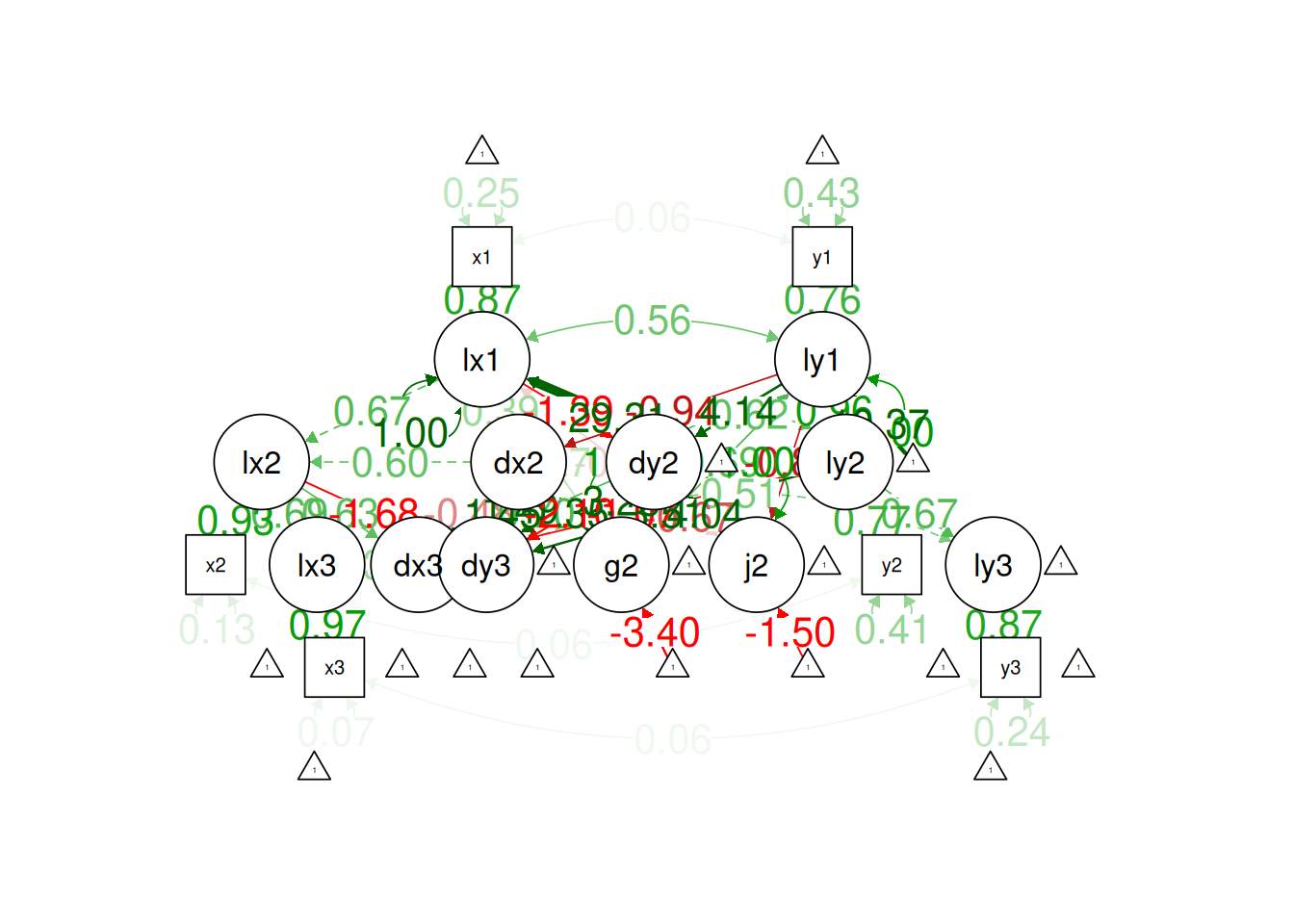
lcsm::plot_lcsm(
  lavaan_object = bivariateLCSM_fit,
  lcsm = "bivariate",
  lavaan_syntax = bivariateLCSM_syntax,
  edge.label.cex = .9,
  lcsm_colours = TRUE)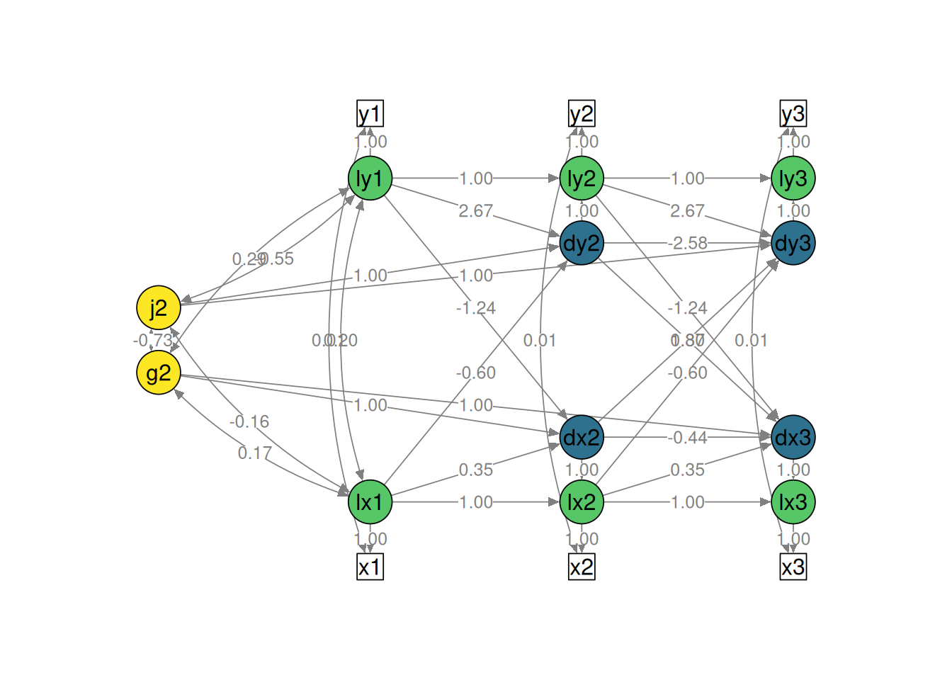
#lavaanPlot::lavaanPlot( # throws error
#  bivariateLCSM_fit,
#  coefs = TRUE,
#  #covs = TRUE,
#  stand = TRUE)

lavaanPlot::lavaanPlot2(
  bivariateLCSM_fit,
  stand = TRUE,
  coef_labels = TRUE)
To generate an interactive/modifiable path diagram, you can use the following syntax:
lavaangui::plot_lavaan(bivariateLCSM_fit)lcsm::plot_trajectories(
data_bi_lcsm,
id_var = "id",
var_list = c(
"x1", "x2", "x3", "x4", "x5",
"x6", "x7", "x8", "x9", "x10"),
xlab = "Time",
ylab = "X Score",
connect_missing = FALSE)
lcsm::plot_trajectories(
  data_bi_lcsm,
  id_var = "id",
  var_list = c(
    "y1", "y2", "y3", "y4", "y5",
    "y6", "y7", "y8", "y9", "y10"),
  xlab = "Time",
  ylab = "Y Score",
  connect_missing = FALSE)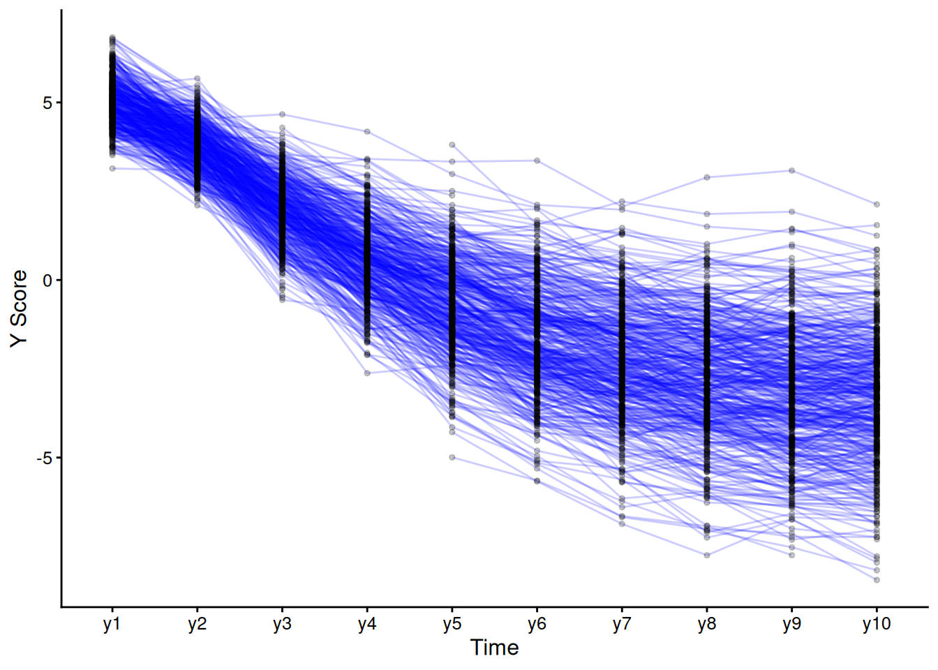
clpm_syntax <- '
  # Autoregressive Paths
  t4 ~ t3
  t3 ~ t2
  t2 ~ t1

  c4 ~ c3
  c3 ~ c2
  c2 ~ c1

  # Concurrent Covariances
  t1 ~~ c1
  t2 ~~ c2
  t3 ~~ c3
  t4 ~~ c4

  # Cross-Lagged Paths
  t4 ~ c3
  t3 ~ c2
  t2 ~ c1

  c4 ~ t3
  c3 ~ t2
  c2 ~ t1
'clpm_fit <- sem(
clpm_syntax,
data = Demo.growth,
missing = "ML",
estimator = "MLR",
meanstructure = TRUE,
std.lv = TRUE,
fixed.x = FALSE,
em.h1.iter.max = 100000)summary(
clpm_fit,
fit.measures = TRUE,
standardized = TRUE,
rsquare = TRUE)lavaan 0.6-21 ended normally after 25 iterations
Estimator ML
Optimization method NLMINB
Number of model parameters 32
Number of observations 400
Number of missing patterns 1
Model Test User Model:
Standard Scaled
Test Statistic 55.624 54.099
Degrees of freedom 12 12
P-value (Chi-square) 0.000 0.000
Scaling correction factor 1.028
Yuan-Bentler correction (Mplus variant)
Model Test Baseline Model:
Test statistic 1933.670 1953.262
Degrees of freedom 28 28
P-value 0.000 0.000
Scaling correction factor 0.990
User Model versus Baseline Model:
Comparative Fit Index (CFI) 0.977 0.978
Tucker-Lewis Index (TLI) 0.947 0.949
Robust Comparative Fit Index (CFI) 0.977
Robust Tucker-Lewis Index (TLI) 0.947
Loglikelihood and Information Criteria:
Loglikelihood user model (H0) -4885.800 -4885.800
Scaling correction factor 1.001
for the MLR correction
Loglikelihood unrestricted model (H1) -4857.988 -4857.988
Scaling correction factor 1.008
for the MLR correction
Akaike (AIC) 9835.601 9835.601
Bayesian (BIC) 9963.328 9963.328
Sample-size adjusted Bayesian (SABIC) 9861.790 9861.790
Root Mean Square Error of Approximation:
RMSEA 0.095 0.094
90 Percent confidence interval - lower 0.071 0.069
90 Percent confidence interval - upper 0.121 0.119
P-value H_0: RMSEA <= 0.050 0.002 0.002
P-value H_0: RMSEA >= 0.080 0.856 0.832
Robust RMSEA 0.095
90 Percent confidence interval - lower 0.070
90 Percent confidence interval - upper 0.121
P-value H_0: Robust RMSEA <= 0.050 0.002
P-value H_0: Robust RMSEA >= 0.080 0.849
Standardized Root Mean Square Residual:
SRMR 0.029 0.029
Parameter Estimates:
Standard errors Sandwich
Information bread Observed
Observed information based on Hessian
Regressions:
Estimate Std.Err z-value P(>|z|) Std.lv Std.all
t4 ~
t3 1.183 0.023 51.960 0.000 1.183 0.954
t3 ~
t2 1.135 0.031 36.564 0.000 1.135 0.885
t2 ~
t1 1.040 0.047 21.910 0.000 1.040 0.773
c4 ~
c3 0.063 0.051 1.227 0.220 0.063 0.063
c3 ~
c2 -0.015 0.046 -0.319 0.750 -0.015 -0.015
c2 ~
c1 0.081 0.046 1.761 0.078 0.081 0.084
t4 ~
c3 -0.323 0.065 -4.935 0.000 -0.323 -0.089
t3 ~
c2 -0.336 0.069 -4.838 0.000 -0.336 -0.117
t2 ~
c1 -0.114 0.065 -1.749 0.080 -0.114 -0.053
c4 ~
t3 -0.030 0.018 -1.717 0.086 -0.030 -0.089
c3 ~
t2 0.053 0.022 2.377 0.017 0.053 0.121
c2 ~
t1 0.009 0.029 0.328 0.743 0.009 0.016
Covariances:
Estimate Std.Err z-value P(>|z|) Std.lv Std.all
t1 ~~
c1 0.114 0.081 1.408 0.159 0.114 0.073
.t2 ~~
.c2 0.244 0.064 3.798 0.000 0.244 0.191
.t3 ~~
.c3 0.376 0.072 5.224 0.000 0.376 0.310
.t4 ~~
.c4 0.268 0.055 4.913 0.000 0.268 0.246
Intercepts:
Estimate Std.Err z-value P(>|z|) Std.lv Std.all
.t4 0.593 0.083 7.110 0.000 0.593 0.176
.t3 0.704 0.086 8.145 0.000 0.704 0.259
.t2 1.056 0.071 14.794 0.000 1.056 0.497
.c4 0.056 0.067 0.835 0.404 0.056 0.061
.c3 -0.021 0.060 -0.351 0.725 -0.021 -0.023
.c2 0.023 0.049 0.465 0.642 0.023 0.024
t1 0.595 0.079 7.531 0.000 0.595 0.377
c1 0.008 0.049 0.158 0.874 0.008 0.008
Variances:
Estimate Std.Err z-value P(>|z|) Std.lv Std.all
.t4 1.416 0.092 15.404 0.000 1.416 0.124
.t3 1.703 0.125 13.598 0.000 1.703 0.230
.t2 1.825 0.137 13.275 0.000 1.825 0.405
.c4 0.844 0.056 15.195 0.000 0.844 0.991
.c3 0.859 0.065 13.252 0.000 0.859 0.986
.c2 0.892 0.061 14.608 0.000 0.892 0.992
t1 2.494 0.185 13.450 0.000 2.494 1.000
c1 0.972 0.063 15.321 0.000 0.972 1.000
R-Square:
Estimate
t4 0.876
t3 0.770
t2 0.595
c4 0.009
c3 0.014
c2 0.008fitMeasures(
clpm_fit,
fit.measures = c(
"chisq", "df", "pvalue",
"chisq.scaled", "df.scaled", "pvalue.scaled",
"chisq.scaling.factor",
"baseline.chisq","baseline.df","baseline.pvalue",
"rmsea", "cfi", "tli", "srmr",
"rmsea.robust", "cfi.robust", "tli.robust")) chisq df pvalue
55.624 12.000 0.000
chisq.scaled df.scaled pvalue.scaled
54.099 12.000 0.000
chisq.scaling.factor baseline.chisq baseline.df
1.028 1933.670 28.000
baseline.pvalue rmsea cfi
0.000 0.095 0.977
tli srmr rmsea.robust
0.947 0.029 0.095
cfi.robust tli.robust
0.977 0.947 residuals(
clpm_fit,
type = "cor")$type
[1] "cor.bollen"
$cov
t4 t3 t2 c4 c3 c2 t1 c1
t4 0.000
t3 0.000 0.000
t2 0.044 0.000 0.000
c4 0.000 0.000 0.030 0.000
c3 0.000 0.000 0.000 0.000 0.000
c2 0.005 0.000 0.000 0.036 0.000 0.000
t1 0.068 0.038 0.000 0.052 0.024 0.000 0.000
c1 0.048 -0.022 0.000 0.140 -0.032 0.000 0.000 0.000
$mean
t4 t3 t2 c4 c3 c2 t1 c1
0 0 0 0 0 0 0 0 modificationindices(
clpm_fit,
sort. = TRUE)semPaths(
clpm_fit,
what = "Std.all",
layout = "tree2",
edge.label.cex = 1.5)
lavaanPlot::lavaanPlot(
  clpm_fit,
  coefs = TRUE,
  #covs = TRUE,
stand = TRUE)lavaanPlot::lavaanPlot2(
clpm_fit,
#stand = TRUE, # currently throws error; uncomment out when fixed: https://github.com/alishinski/lavaanPlot/issues/52
coef_labels = TRUE)To generate an interactive/modifiable path diagram, you can use the following syntax:
lavaangui::plot_lavaan(clpm_fit)Adapted from Mulder & Hamaker (2021): https://doi.org/10.1080/10705511.2020.1784738
https://jeroendmulder.github.io/RI-CLPM/lavaan.html (archived at https://perma.cc/2K6A-WUJQ)
riclpm1_syntax <- '
  # Random Intercepts
  t =~ 1*t1 + 1*t2 + 1*t3 + 1*t4
  c =~ 1*c1 + 1*c2 + 1*c3 + 1*c4

  # Create Within-Person Centered Variables
  wt1 =~ 1*t1
  wt2 =~ 1*t2
  wt3 =~ 1*t3
  wt4 =~ 1*t4

  wc1 =~ 1*c1
  wc2 =~ 1*c2
  wc3 =~ 1*c3
  wc4 =~ 1*c4

  # Autoregressive Paths
  wt4 ~ wt3
  wt3 ~ wt2
  wt2 ~ wt1

  wc4 ~ wc3
  wc3 ~ wc2
  wc2 ~ wc1

  # Concurrent Covariances
  wt1 ~~ wc1
  wt2 ~~ wc2
  wt3 ~~ wc3
  wt4 ~~ wc4

  # Cross-Lagged Paths
  wt4 ~ wc3
  wt3 ~ wc2
  wt2 ~ wc1

  wc4 ~ wt3
  wc3 ~ wt2
  wc2 ~ wt1

  # Variance and Covariance of Random Intercepts
  t ~~ t
  c ~~ c
  t ~~ c

  # Variances of Within-Person Centered Variables
  wt1 ~~ wt1
  wt2 ~~ wt2
  wt3 ~~ wt3
  wt4 ~~ wt4

  wc1 ~~ wc1
  wc2 ~~ wc2
  wc3 ~~ wc3
  wc4 ~~ wc4
'Adapted from Mund & Nestler (2017): https://osf.io/a4dhk
riclpm2_syntax <- '
  # Random Intercepts
  t =~ 1*t1 + 1*t2 + 1*t3 + 1*t4
  c =~ 1*c1 + 1*c2 + 1*c3 + 1*c4

  # Create Within-Person Centered Variables
  wt1 =~ 1*t1
  wt2 =~ 1*t2
  wt3 =~ 1*t3
  wt4 =~ 1*t4

  wc1 =~ 1*c1
  wc2 =~ 1*c2
  wc3 =~ 1*c3
  wc4 =~ 1*c4

  # Autoregressive Paths
  wt4 ~ wt3
  wt3 ~ wt2
  wt2 ~ wt1

  wc4 ~ wc3
  wc3 ~ wc2
  wc2 ~ wc1

  # Concurrent Covariances
  wt1 ~~ wc1
  wt2 ~~ wc2
  wt3 ~~ wc3
  wt4 ~~ wc4

  # Cross-Lagged Paths
  wt4 ~ wc3
  wt3 ~ wc2
  wt2 ~ wc1

  wc4 ~ wt3
  wc3 ~ wt2
  wc2 ~ wt1

  # Variance and Covariance of Random Intercepts
  t ~~ t
  c ~~ c
  t ~~ c

  # Variances of Within-Person Centered Variables
  wt1 ~~ wt1
  wt2 ~~ wt2
  wt3 ~~ wt3
  wt4 ~~ wt4

  wc1 ~~ wc1
  wc2 ~~ wc2
  wc3 ~~ wc3
  wc4 ~~ wc4

  # Fix Error Variances of Observed Variables to Zero
  t1 ~~ 0*t1
  t2 ~~ 0*t2
  t3 ~~ 0*t3
  t4 ~~ 0*t4

  c1 ~~ 0*c1
  c2 ~~ 0*c2
  c3 ~~ 0*c3
  c4 ~~ 0*c4

  # Fix the Covariances Between the Random Intercepts and the Latents at T1 to Zero
  wt1 ~~ 0*t
  wt1 ~~ 0*c

  wc1 ~~ 0*t
  wc1 ~~ 0*c

  # Estimate Observed Intercepts
  t1 ~ 1
  t2 ~ 1
  t3 ~ 1
  t4 ~ 1

  c1 ~ 1
  c2 ~ 1
  c3 ~ 1
  c4 ~ 1

  # Fix the Means of the Latents to Zero
  wt1 ~ 0*1
  wt2 ~ 0*1
  wt3 ~ 0*1
  wt4 ~ 0*1

  wc1 ~ 0*1
  wc2 ~ 0*1
  wc3 ~ 0*1
  wc4 ~ 0*1

  t ~ 0*1
  c ~ 0*1
'riclpm1_fit <- lavaan(
riclpm1_syntax,
data = Demo.growth,
missing = "ML",
estimator = "MLR",
meanstructure = TRUE,
int.ov.free = TRUE,
fixed.x = FALSE,
em.h1.iter.max = 100000)riclpm2_fit <- sem(
riclpm2_syntax,
data = Demo.growth,
missing = "ML",
estimator = "MLR",
fixed.x = FALSE,
em.h1.iter.max = 100000)summary(
riclpm1_fit,
fit.measures = TRUE,
standardized = TRUE,
rsquare = TRUE)lavaan 0.6-21 ended normally after 63 iterations
Estimator ML
Optimization method NLMINB
Number of model parameters 35
Number of observations 400
Number of missing patterns 1
Model Test User Model:
Standard Scaled
Test Statistic 39.156 38.001
Degrees of freedom 9 9
P-value (Chi-square) 0.000 0.000
Scaling correction factor 1.030
Yuan-Bentler correction (Mplus variant)
Model Test Baseline Model:
Test statistic 1933.670 1953.262
Degrees of freedom 28 28
P-value 0.000 0.000
Scaling correction factor 0.990
User Model versus Baseline Model:
Comparative Fit Index (CFI) 0.984 0.985
Tucker-Lewis Index (TLI) 0.951 0.953
Robust Comparative Fit Index (CFI) 0.984
Robust Tucker-Lewis Index (TLI) 0.951
Loglikelihood and Information Criteria:
Loglikelihood user model (H0) -4877.566 -4877.566
Scaling correction factor 1.003
for the MLR correction
Loglikelihood unrestricted model (H1) -4857.988 -4857.988
Scaling correction factor 1.008
for the MLR correction
Akaike (AIC) 9825.132 9825.132
Bayesian (BIC) 9964.833 9964.833
Sample-size adjusted Bayesian (SABIC) 9853.776 9853.776
Root Mean Square Error of Approximation:
RMSEA 0.092 0.090
90 Percent confidence interval - lower 0.063 0.062
90 Percent confidence interval - upper 0.122 0.120
P-value H_0: RMSEA <= 0.050 0.009 0.011
P-value H_0: RMSEA >= 0.080 0.766 0.737
Robust RMSEA 0.091
90 Percent confidence interval - lower 0.062
90 Percent confidence interval - upper 0.122
P-value H_0: Robust RMSEA <= 0.050 0.011
P-value H_0: Robust RMSEA >= 0.080 0.756
Standardized Root Mean Square Residual:
SRMR 0.023 0.023
Parameter Estimates:
Standard errors Sandwich
Information bread Observed
Observed information based on Hessian
Latent Variables:
Estimate Std.Err z-value P(>|z|) Std.lv Std.all
t =~
t1 1.000 NA NA
t2 1.000 NA NA
t3 1.000 NA NA
t4 1.000 NA NA
c =~
c1 1.000 0.206 0.209
c2 1.000 0.206 0.217
c3 1.000 0.206 0.220
c4 1.000 0.206 0.224
wt1 =~
t1 1.000 2.318 1.462
wt2 =~
t2 1.000 2.695 1.284
wt3 =~
t3 1.000 3.219 1.175
wt4 =~
t4 1.000 3.786 1.118
wc1 =~
c1 1.000 0.965 0.978
wc2 =~
c2 1.000 0.927 0.976
wc3 =~
c3 1.000 0.915 0.976
wc4 =~
c4 1.000 0.894 0.975
Regressions:
Estimate Std.Err z-value P(>|z|) Std.lv Std.all
wt4 ~
wt3 1.126 0.029 38.930 0.000 0.957 0.957
wt3 ~
wt2 1.093 0.025 43.596 0.000 0.915 0.915
wt2 ~
wt1 1.005 0.025 40.746 0.000 0.864 0.864
wc4 ~
wc3 0.004 0.061 0.063 0.950 0.004 0.004
wc3 ~
wc2 -0.047 0.056 -0.839 0.401 -0.048 -0.048
wc2 ~
wc1 0.042 0.051 0.816 0.415 0.043 0.043
wt4 ~
wc3 -0.291 0.076 -3.838 0.000 -0.070 -0.070
wt3 ~
wc2 -0.326 0.074 -4.413 0.000 -0.094 -0.094
wt2 ~
wc1 -0.113 0.068 -1.661 0.097 -0.041 -0.041
wc4 ~
wt3 -0.021 0.020 -1.044 0.296 -0.075 -0.075
wc3 ~
wt2 0.020 0.023 0.881 0.378 0.059 0.059
wc2 ~
wt1 -0.010 0.024 -0.420 0.675 -0.025 -0.025
Covariances:
Estimate Std.Err z-value P(>|z|) Std.lv Std.all
wt1 ~~
wc1 -0.007 0.136 -0.054 0.957 -0.003 -0.003
.wt2 ~~
.wc2 0.242 0.064 3.775 0.000 0.193 0.193
.wt3 ~~
.wc3 0.385 0.074 5.191 0.000 0.322 0.322
.wt4 ~~
.wc4 0.238 0.058 4.071 0.000 0.219 0.219
t ~~
c 0.082 0.107 0.761 0.447 0.235 0.235
Intercepts:
Estimate Std.Err z-value P(>|z|) Std.lv Std.all
.t1 0.595 0.079 7.531 0.000 0.595 0.375
.t2 1.673 0.106 15.763 0.000 1.673 0.797
.t3 2.593 0.136 19.058 0.000 2.593 0.947
.t4 3.639 0.169 21.572 0.000 3.639 1.074
.c1 0.008 0.049 0.158 0.874 0.008 0.008
.c2 0.029 0.047 0.610 0.542 0.029 0.030
.c3 0.068 0.047 1.449 0.147 0.068 0.072
.c4 -0.018 0.046 -0.390 0.696 -0.018 -0.020
Variances:
Estimate Std.Err z-value P(>|z|) Std.lv Std.all
t -2.861 1.350 -2.119 0.034 NA NA
c 0.042 0.026 1.637 0.102 1.000 1.000
wt1 5.373 1.412 3.804 0.000 1.000 1.000
.wt2 1.829 0.138 13.209 0.000 0.252 0.252
.wt3 1.719 0.127 13.564 0.000 0.166 0.166
.wt4 1.484 0.097 15.331 0.000 0.103 0.103
wc1 0.931 0.067 13.826 0.000 1.000 1.000
.wc2 0.856 0.065 13.256 0.000 0.997 0.997
.wc3 0.832 0.070 11.817 0.000 0.995 0.995
.wc4 0.795 0.061 13.110 0.000 0.994 0.994
.t1 0.000 0.000 0.000
.t2 0.000 0.000 0.000
.t3 0.000 0.000 0.000
.t4 0.000 0.000 0.000
.c1 0.000 0.000 0.000
.c2 0.000 0.000 0.000
.c3 0.000 0.000 0.000
.c4 0.000 0.000 0.000
R-Square:
Estimate
wt2 0.748
wt3 0.834
wt4 0.897
wc2 0.003
wc3 0.005
wc4 0.006
t1 1.000
t2 1.000
t3 1.000
t4 1.000
c1 1.000
c2 1.000
c3 1.000
c4 1.000summary(
riclpm2_fit,
fit.measures = TRUE,
standardized = TRUE,
rsquare = TRUE)lavaan 0.6-21 ended normally after 63 iterations
Estimator ML
Optimization method NLMINB
Number of model parameters 35
Number of observations 400
Number of missing patterns 1
Model Test User Model:
Standard Scaled
Test Statistic 39.156 38.001
Degrees of freedom 9 9
P-value (Chi-square) 0.000 0.000
Scaling correction factor 1.030
Yuan-Bentler correction (Mplus variant)
Model Test Baseline Model:
Test statistic 1933.670 1953.262
Degrees of freedom 28 28
P-value 0.000 0.000
Scaling correction factor 0.990
User Model versus Baseline Model:
Comparative Fit Index (CFI) 0.984 0.985
Tucker-Lewis Index (TLI) 0.951 0.953
Robust Comparative Fit Index (CFI) 0.984
Robust Tucker-Lewis Index (TLI) 0.951
Loglikelihood and Information Criteria:
Loglikelihood user model (H0) -4877.566 -4877.566
Scaling correction factor 1.003
for the MLR correction
Loglikelihood unrestricted model (H1) -4857.988 -4857.988
Scaling correction factor 1.008
for the MLR correction
Akaike (AIC) 9825.132 9825.132
Bayesian (BIC) 9964.833 9964.833
Sample-size adjusted Bayesian (SABIC) 9853.776 9853.776
Root Mean Square Error of Approximation:
RMSEA 0.092 0.090
90 Percent confidence interval - lower 0.063 0.062
90 Percent confidence interval - upper 0.122 0.120
P-value H_0: RMSEA <= 0.050 0.009 0.011
P-value H_0: RMSEA >= 0.080 0.766 0.737
Robust RMSEA 0.091
90 Percent confidence interval - lower 0.062
90 Percent confidence interval - upper 0.122
P-value H_0: Robust RMSEA <= 0.050 0.011
P-value H_0: Robust RMSEA >= 0.080 0.756
Standardized Root Mean Square Residual:
SRMR 0.023 0.023
Parameter Estimates:
Standard errors Sandwich
Information bread Observed
Observed information based on Hessian
Latent Variables:
Estimate Std.Err z-value P(>|z|) Std.lv Std.all
t =~
t1 1.000 NA NA
t2 1.000 NA NA
t3 1.000 NA NA
t4 1.000 NA NA
c =~
c1 1.000 0.206 0.209
c2 1.000 0.206 0.217
c3 1.000 0.206 0.220
c4 1.000 0.206 0.224
wt1 =~
t1 1.000 2.318 1.462
wt2 =~
t2 1.000 2.695 1.284
wt3 =~
t3 1.000 3.219 1.175
wt4 =~
t4 1.000 3.786 1.118
wc1 =~
c1 1.000 0.965 0.978
wc2 =~
c2 1.000 0.927 0.976
wc3 =~
c3 1.000 0.915 0.976
wc4 =~
c4 1.000 0.894 0.975
Regressions:
Estimate Std.Err z-value P(>|z|) Std.lv Std.all
wt4 ~
wt3 1.126 0.029 38.930 0.000 0.957 0.957
wt3 ~
wt2 1.093 0.025 43.596 0.000 0.915 0.915
wt2 ~
wt1 1.005 0.025 40.746 0.000 0.864 0.864
wc4 ~
wc3 0.004 0.061 0.063 0.950 0.004 0.004
wc3 ~
wc2 -0.047 0.056 -0.839 0.401 -0.048 -0.048
wc2 ~
wc1 0.042 0.051 0.816 0.415 0.043 0.043
wt4 ~
wc3 -0.291 0.076 -3.838 0.000 -0.070 -0.070
wt3 ~
wc2 -0.326 0.074 -4.413 0.000 -0.094 -0.094
wt2 ~
wc1 -0.113 0.068 -1.661 0.097 -0.041 -0.041
wc4 ~
wt3 -0.021 0.020 -1.044 0.296 -0.075 -0.075
wc3 ~
wt2 0.020 0.023 0.881 0.378 0.059 0.059
wc2 ~
wt1 -0.010 0.024 -0.420 0.675 -0.025 -0.025
Covariances:
Estimate Std.Err z-value P(>|z|) Std.lv Std.all
wt1 ~~
wc1 -0.007 0.136 -0.054 0.957 -0.003 -0.003
.wt2 ~~
.wc2 0.242 0.064 3.775 0.000 0.193 0.193
.wt3 ~~
.wc3 0.385 0.074 5.191 0.000 0.322 0.322
.wt4 ~~
.wc4 0.238 0.058 4.071 0.000 0.219 0.219
t ~~
c 0.082 0.107 0.761 0.447 0.235 0.235
wt1 0.000 0.000 0.000
c ~~
wt1 0.000 0.000 0.000
t ~~
wc1 0.000 0.000 0.000
c ~~
wc1 0.000 0.000 0.000
Intercepts:
Estimate Std.Err z-value P(>|z|) Std.lv Std.all
.t1 0.595 0.079 7.531 0.000 0.595 0.375
.t2 1.673 0.106 15.763 0.000 1.673 0.797
.t3 2.593 0.136 19.058 0.000 2.593 0.947
.t4 3.639 0.169 21.572 0.000 3.639 1.074
.c1 0.008 0.049 0.158 0.874 0.008 0.008
.c2 0.029 0.047 0.610 0.542 0.029 0.030
.c3 0.068 0.047 1.449 0.147 0.068 0.072
.c4 -0.018 0.046 -0.390 0.696 -0.018 -0.020
wt1 0.000 0.000 0.000
.wt2 0.000 0.000 0.000
.wt3 0.000 0.000 0.000
.wt4 0.000 0.000 0.000
wc1 0.000 0.000 0.000
.wc2 0.000 0.000 0.000
.wc3 0.000 0.000 0.000
.wc4 0.000 0.000 0.000
t 0.000 NA NA
c 0.000 0.000 0.000
Variances:
Estimate Std.Err z-value P(>|z|) Std.lv Std.all
t -2.861 1.350 -2.119 0.034 NA NA
c 0.042 0.026 1.637 0.102 1.000 1.000
wt1 5.373 1.412 3.804 0.000 1.000 1.000
.wt2 1.829 0.138 13.209 0.000 0.252 0.252
.wt3 1.719 0.127 13.564 0.000 0.166 0.166
.wt4 1.484 0.097 15.331 0.000 0.103 0.103
wc1 0.931 0.067 13.826 0.000 1.000 1.000
.wc2 0.856 0.065 13.256 0.000 0.997 0.997
.wc3 0.832 0.070 11.817 0.000 0.995 0.995
.wc4 0.795 0.061 13.110 0.000 0.994 0.994
.t1 0.000 0.000 0.000
.t2 0.000 0.000 0.000
.t3 0.000 0.000 0.000
.t4 0.000 0.000 0.000
.c1 0.000 0.000 0.000
.c2 0.000 0.000 0.000
.c3 0.000 0.000 0.000
.c4 0.000 0.000 0.000
R-Square:
Estimate
wt2 0.748
wt3 0.834
wt4 0.897
wc2 0.003
wc3 0.005
wc4 0.006
t1 1.000
t2 1.000
t3 1.000
t4 1.000
c1 1.000
c2 1.000
c3 1.000
c4 1.000fitMeasures(
riclpm1_fit,
fit.measures = c(
"chisq", "df", "pvalue",
"chisq.scaled", "df.scaled", "pvalue.scaled",
"chisq.scaling.factor",
"baseline.chisq","baseline.df","baseline.pvalue",
"rmsea", "cfi", "tli", "srmr",
"rmsea.robust", "cfi.robust", "tli.robust")) chisq df pvalue
39.156 9.000 0.000
chisq.scaled df.scaled pvalue.scaled
38.001 9.000 0.000
chisq.scaling.factor baseline.chisq baseline.df
1.030 1933.670 28.000
baseline.pvalue rmsea cfi
0.000 0.092 0.984
tli srmr rmsea.robust
0.951 0.023 0.091
cfi.robust tli.robust
0.984 0.951 residuals(
riclpm1_fit,
type = "cor")$type
[1] "cor.bollen"
$cov
t1 t2 t3 t4 c1 c2 c3 c4
t1 0.000
t2 0.007 0.000
t3 0.012 -0.004 0.000
t4 0.005 0.023 0.000 0.000
c1 0.025 0.018 -0.009 0.062 0.000
c2 0.003 0.000 0.000 0.005 -0.001 0.000
c3 -0.013 0.008 0.008 0.009 -0.074 -0.005 0.000
c4 0.026 0.003 -0.020 -0.013 0.090 -0.014 0.001 0.000
$mean
t1 t2 t3 t4 c1 c2 c3 c4
0 0 0 0 0 0 0 0 modificationindices(
riclpm1_fit,
sort. = TRUE)compRelSEM(riclpm1_fit)$t
Composite `t` is composed of observed variables:
t1, t2, t3, t4
True-score variance is represented by common factor(s):
wt1, wt2, wt3, wc1, wc2, wc3
Total variance of composite `t` determined from the unrestricted model.
The proportion attributable to "true" scores is its model-based estimate of reliability ("omega"):
[1] 0.851
$c
Composite `c` is composed of observed variables:
c1, c2, c3, c4
True-score variance is represented by common factor(s):
wt1, wt2, wt3, wc1, wc2, wc3
Total variance of composite `c` determined from the unrestricted model.
The proportion attributable to "true" scores is its model-based estimate of reliability ("omega"):
[1] 0.001semPaths(
riclpm1_fit,
what = "Std.all",
layout = "tree2",
edge.label.cex = 1.5)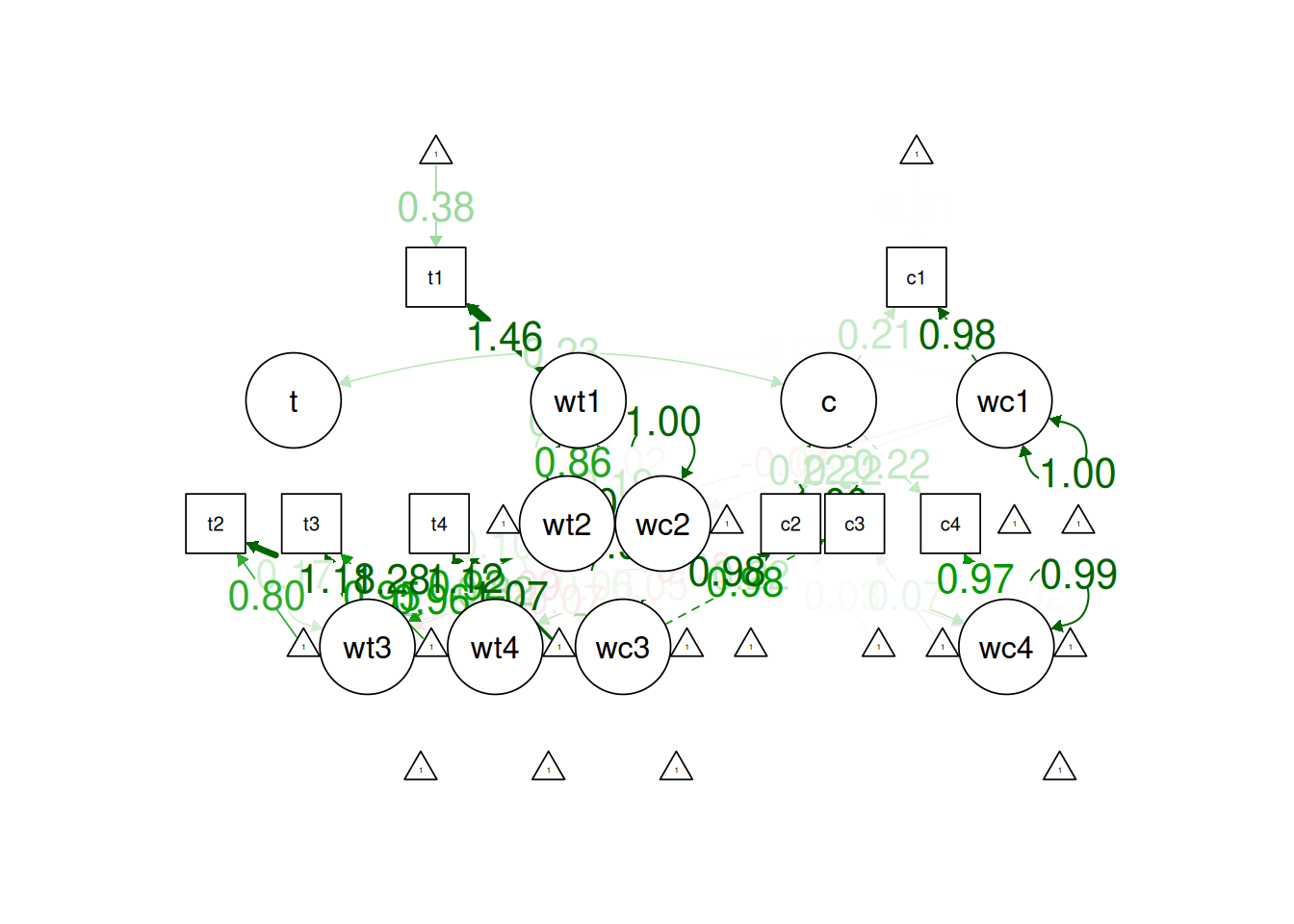
lavaanPlot::lavaanPlot(
  riclpm1_fit,
  coefs = TRUE,
  #covs = TRUE,
stand = TRUE)lavaanPlot::lavaanPlot2(
riclpm1_fit,
#stand = TRUE, # currently throws error; uncomment out when fixed: https://github.com/alishinski/lavaanPlot/issues/52
coef_labels = TRUE)To generate an interactive/modifiable path diagram, you can use the following syntax:
lavaangui::plot_lavaan(riclpm1_fit)As noted by Curran and Hancock (2021) and in their corresponding episode on Quantitude, in an ALT model, the time-linked relations affect the underlying growth trajectories and vice versa, thus preventing the pure isolation of within-person and between-person effects. Thus, researchers advocate for the use of the latent curve model with structured residuals (LCM-SR) to separate within-person and between-person effects.
alt_syntax <- '
  # Intercept and slope
  intercept_t =~ 1*t1 + 1*t2 + 1*t3 + 1*t4
  slope_t =~ 0*t1 + 1*t2 + 2*t3 + 3*t4

  intercept_c =~ 1*c1 + 1*c2 + 1*c3 + 1*c4
  slope_c =~ 0*c1 + 1*c2 + 2*c3 + 3*c4

  # Autoregressive Paths
  t4 ~ t3
  t3 ~ t2
  t2 ~ t1

  c4 ~ c3
  c3 ~ c2
  c2 ~ c1

  # Concurrent Covariances
  t1 ~~ c1
  t2 ~~ c2
  t3 ~~ c3
  t4 ~~ c4

  # Cross-Lagged Paths
  t4 ~ c3
  t3 ~ c2
  t2 ~ c1

  c4 ~ t3
  c3 ~ t2
  c2 ~ t1
'alt_fit <- sem(
alt_syntax,
data = Demo.growth,
missing = "ML",
estimator = "MLR",
fixed.x = FALSE,
em.h1.iter.max = 100000)summary(
alt_fit,
fit.measures = TRUE,
standardized = TRUE,
rsquare = TRUE)lavaan 0.6-21 ended normally after 98 iterations
Estimator ML
Optimization method NLMINB
Number of model parameters 42
Number of observations 400
Number of missing patterns 1
Model Test User Model:
Standard Scaled
Test Statistic 4.176 7.740
Degrees of freedom 2 2
P-value (Chi-square) 0.124 0.021
Scaling correction factor 0.540
Yuan-Bentler correction (Mplus variant)
Model Test Baseline Model:
Test statistic 1933.670 1953.262
Degrees of freedom 28 28
P-value 0.000 0.000
Scaling correction factor 0.990
User Model versus Baseline Model:
Comparative Fit Index (CFI) 0.999 0.997
Tucker-Lewis Index (TLI) 0.984 0.958
Robust Comparative Fit Index (CFI) 0.999
Robust Tucker-Lewis Index (TLI) 0.984
Loglikelihood and Information Criteria:
Loglikelihood user model (H0) -4860.076 -4860.076
Scaling correction factor 1.031
for the MLR correction
Loglikelihood unrestricted model (H1) -4857.988 -4857.988
Scaling correction factor 1.008
for the MLR correction
Akaike (AIC) 9804.152 9804.152
Bayesian (BIC) 9971.794 9971.794
Sample-size adjusted Bayesian (SABIC) 9838.525 9838.525
Root Mean Square Error of Approximation:
RMSEA 0.052 0.085
90 Percent confidence interval - lower 0.000 0.009
90 Percent confidence interval - upper 0.124 0.177
P-value H_0: RMSEA <= 0.050 0.376 0.166
P-value H_0: RMSEA >= 0.080 0.322 0.640
Robust RMSEA 0.051
90 Percent confidence interval - lower 0.000
90 Percent confidence interval - upper 0.124
P-value H_0: Robust RMSEA <= 0.050 0.382
P-value H_0: Robust RMSEA >= 0.080 0.322
Standardized Root Mean Square Residual:
SRMR 0.009 0.009
Parameter Estimates:
Standard errors Sandwich
Information bread Observed
Observed information based on Hessian
Latent Variables:
Estimate Std.Err z-value P(>|z|) Std.lv Std.all
intercept_t =~
t1 1.000 1.124 0.709
t2 1.000 1.124 0.529
t3 1.000 1.124 0.413
t4 1.000 1.124 0.333
slope_t =~
t1 0.000 0.000 0.000
t2 1.000 0.283 0.133
t3 2.000 0.566 0.208
t4 3.000 0.848 0.252
intercept_c =~
c1 1.000 NA NA
c2 1.000 NA NA
c3 1.000 NA NA
c4 1.000 NA NA
slope_c =~
c1 0.000 NA NA
c2 1.000 NA NA
c3 2.000 NA NA
c4 3.000 NA NA
Regressions:
Estimate Std.Err z-value P(>|z|) Std.lv Std.all
t4 ~
t3 0.420 0.342 1.230 0.219 0.420 0.339
t3 ~
t2 0.380 0.302 1.259 0.208 0.380 0.297
t2 ~
t1 0.359 0.254 1.415 0.157 0.359 0.267
c4 ~
c3 0.139 0.187 0.746 0.456 0.139 0.141
c3 ~
c2 0.041 0.153 0.269 0.788 0.041 0.042
c2 ~
c1 0.250 0.195 1.281 0.200 0.250 0.258
t4 ~
c3 0.357 0.183 1.958 0.050 0.357 0.099
t3 ~
c2 0.027 0.145 0.184 0.854 0.027 0.009
t2 ~
c1 0.250 0.207 1.206 0.228 0.250 0.115
c4 ~
t3 0.235 0.229 1.028 0.304 0.235 0.690
c3 ~
t2 0.285 0.208 1.373 0.170 0.285 0.649
c2 ~
t1 0.228 0.186 1.226 0.220 0.228 0.381
Covariances:
Estimate Std.Err z-value P(>|z|) Std.lv Std.all
.t1 ~~
.c1 0.615 0.367 1.674 0.094 0.615 0.479
.t2 ~~
.c2 0.499 0.304 1.643 0.100 0.499 0.485
.t3 ~~
.c3 0.641 0.271 2.366 0.018 0.641 0.608
.t4 ~~
.c4 0.821 0.525 1.565 0.118 0.821 0.687
intercept_t ~~
slope_t 0.392 0.204 1.925 0.054 1.233 1.233
intercept_c -0.498 0.368 -1.352 0.176 -0.738 -0.738
slope_c -0.063 0.138 -0.459 0.646 -0.232 -0.232
slope_t ~~
intercept_c 0.212 0.142 1.496 0.135 1.250 1.250
slope_c -0.209 0.100 -2.098 0.036 -3.035 -3.035
intercept_c ~~
slope_c 0.170 0.133 1.277 0.202 1.163 1.163
Intercepts:
Estimate Std.Err z-value P(>|z|) Std.lv Std.all
.t1 0.595 0.079 7.531 0.000 0.595 0.375
.t2 1.458 0.179 8.134 0.000 1.458 0.686
.t3 1.956 0.536 3.652 0.000 1.956 0.719
.t4 2.525 0.905 2.790 0.005 2.525 0.749
.c1 0.008 0.049 0.158 0.874 0.008 0.008
.c2 -0.109 0.119 -0.916 0.360 -0.109 -0.115
.c3 -0.411 0.358 -1.148 0.251 -0.411 -0.440
.c4 -0.638 0.588 -1.084 0.278 -0.638 -0.687
Variances:
Estimate Std.Err z-value P(>|z|) Std.lv Std.all
.t1 1.246 0.493 2.527 0.012 1.246 0.497
.t2 0.943 0.351 2.688 0.007 0.943 0.209
.t3 1.078 0.382 2.823 0.005 1.078 0.146
.t4 1.114 0.631 1.767 0.077 1.114 0.098
.c1 1.321 0.338 3.905 0.000 1.321 1.375
.c2 1.125 0.311 3.619 0.000 1.125 1.252
.c3 1.030 0.251 4.102 0.000 1.030 1.178
.c4 1.282 0.461 2.778 0.005 1.282 1.490
intercept_t 1.263 0.491 2.573 0.010 1.000 1.000
slope_t 0.080 0.287 0.279 0.781 1.000 1.000
intercept_c -0.360 0.325 -1.109 0.268 NA NA
slope_c -0.059 0.063 -0.945 0.345 NA NA
R-Square:
Estimate
t1 0.503
t2 0.791
t3 0.854
t4 0.902
c1 -0.375
c2 -0.252
c3 -0.178
c4 -0.490fitMeasures(
alt_fit,
fit.measures = c(
"chisq", "df", "pvalue",
"chisq.scaled", "df.scaled", "pvalue.scaled",
"chisq.scaling.factor",
"baseline.chisq","baseline.df","baseline.pvalue",
"rmsea", "cfi", "tli", "srmr",
"rmsea.robust", "cfi.robust", "tli.robust")) chisq df pvalue
4.176 2.000 0.124
chisq.scaled df.scaled pvalue.scaled
7.740 2.000 0.021
chisq.scaling.factor baseline.chisq baseline.df
0.540 1933.670 28.000
baseline.pvalue rmsea cfi
0.000 0.052 0.999
tli srmr rmsea.robust
0.984 0.009 0.051
cfi.robust tli.robust
0.999 0.984 residuals(
alt_fit,
type = "cor")$type
[1] "cor.bollen"
$cov
t1 t2 t3 t4 c1 c2 c3 c4
t1 0.000
t2 0.002 0.000
t3 0.014 -0.002 0.000
t4 0.005 0.000 -0.001 0.000
c1 -0.003 0.005 -0.002 0.010 0.000
c2 -0.005 -0.006 -0.008 -0.010 0.003 0.000
c3 0.040 -0.002 0.002 0.001 -0.013 0.000 0.000
c4 -0.030 0.008 0.001 0.002 -0.003 0.005 0.004 0.000
$mean
t1 t2 t3 t4 c1 c2 c3 c4
0 0 0 0 0 0 0 0 modificationindices(
alt_fit,
sort. = TRUE)compRelSEM(alt_fit)Error in `PHI[[b.idx]][myFacNames, myFacNames, drop = FALSE]`:
! subscript out of boundssemPaths(
alt_fit,
what = "Std.all",
layout = "tree2",
edge.label.cex = 1.5)
lavaanPlot::lavaanPlot(
  alt_fit,
  coefs = TRUE,
  #covs = TRUE,
stand = TRUE)lavaanPlot::lavaanPlot2(
alt_fit,
#stand = TRUE, # currently throws error; uncomment out when fixed: https://github.com/alishinski/lavaanPlot/issues/52
coef_labels = TRUE)To generate an interactive/modifiable path diagram, you can use the following syntax:
lavaangui::plot_lavaan(alt_fit)A latent curve model with structured residuals (LCM-SR) is an extension of the autoregressive latent trajectory (ALT) model. A LCM-SR model is also called an autoregressive latent trajectory model with structured residuals (ALT-SR). The LCM-SR separates stable between-person differences in developmental trajectories from within-person deviations around those trajectories. The latent growth factors (e.g., intercept and slope) capture between-person differences, whereas the autoregressive and cross-lagged relations among the structured residuals capture within-person dynamics. A LSM-SR model can also be estimated using multilevel SEM.
Adapted from Mund & Nestler (2017): https://osf.io/a4dhk
lcmsr_syntax <- '
  # Define intercept and growth factors
  intercept.t =~ 1*t1 + 1*t2 + 1*t3 + 1*t4
  slope.t =~ 0*t1 + 1*t2 + 2*t3 + 3*t4

  intercept.c =~ 1*c1 + 1*c2 + 1*c3 + 1*c4
  slope.c =~ 0*c1 + 1*c2 + 2*c3 + 3*c4

  # Define phantom latent variables
  e.t1 =~ 1*t1
  e.t2 =~ 1*t2
  e.t3 =~ 1*t3
  e.t4 =~ 1*t4

  e.c1 =~ 1*c1
  e.c2 =~ 1*c2
  e.c3 =~ 1*c3
  e.c4 =~ 1*c4

  # Autoregressive paths
  e.t2 ~ a1*e.t1
  e.t3 ~ a1*e.t2
  e.t4 ~ a1*e.t3

  e.c2 ~ a2*e.c1
  e.c3 ~ a2*e.c2
  e.c4 ~ a2*e.c3

  # Cross-lagged paths
  e.c2 ~ c1*e.t1
  e.c3 ~ c1*e.t2
  e.c4 ~ c1*e.t3

  e.t2 ~ c2*e.c1
  e.t3 ~ c2*e.c2
  e.t4 ~ c2*e.c3

  # Some further constraints on the variance structure
  # 1. Set error variances of the observed variables to zero
  t1 ~~ 0*t1
  t2 ~~ 0*t2
  t3 ~~ 0*t3
  t4 ~~ 0*t4

  c1 ~~ 0*c1
  c2 ~~ 0*c2
  c3 ~~ 0*c3
  c4 ~~ 0*c4

  # 2. Let lavaan estimate the variance of the latent variables (residuals)
  e.t1 ~~ vart1*e.t1
  e.t2 ~~ vart2*e.t2
  e.t3 ~~ vart3*e.t3
  e.t4 ~~ vart4*e.t4

  e.c1 ~~ varc1*e.c1
  e.c2 ~~ varc2*e.c2
  e.c3 ~~ varc3*e.c3
  e.c4 ~~ varc4*e.c4

  # 3. We also want estimates of the intercept factor variances, the slope
  #    variances, and the covariances
  intercept.t ~~ varintercept.t*intercept.t
  intercept.c ~~ varintercept.c*intercept.c
  slope.t ~~ varslope.t*slope.t
  slope.c ~~ varslope.c*slope.c

  intercept.t ~~ covintercept*intercept.c
  slope.t ~~ covslope*slope.c

  intercept.t ~~ covintercept.tslope.t*slope.t
  intercept.t ~~ covintercept.tslope.c*slope.c
  intercept.c ~~ covintercept.cslope.t*slope.t
  intercept.c ~~ covintercept.cslope.c*slope.c

  # 4. We have to define that the covariance between the intercepts and
  #    the slopes and the latents of the first time point are zero
  e.t1 ~~ 0*intercept.t
  e.c1 ~~ 0*intercept.t
  e.t1 ~~ 0*slope.t
  e.c1 ~~ 0*slope.t
  e.t1 ~~ 0*intercept.c
  e.c1 ~~ 0*intercept.c
  e.t1 ~~ 0*slope.c
  e.c1 ~~ 0*slope.c

  # 5. Finally, we estimate the covariance between the latents of x and y
  #    of the first time point, the second time-point and so on. Note that
  #    for the second to fourth time point the correlation is constrained to
  #    the same value
  e.t1 ~~ cov1*e.c1
  e.t2 ~~ e1*e.c2
  e.t3 ~~ e1*e.c3
  e.t4 ~~ e1*e.c4

  # The model also contains a mean structure and we have to define some
  # constraints for this part of the model. The assumption is that we
  # only want estimates of the mean of the intercept factors. All other means
  # are defined to be zero:
  t1 ~ 0*1
  t2 ~ 0*1
  t3 ~ 0*1
  t4 ~ 0*1

  c1 ~ 0*1
  c2 ~ 0*1
  c3 ~ 0*1
  c4 ~ 0*1

  e.t1 ~ 0*1
  e.t2 ~ 0*1
  e.t3 ~ 0*1
  e.t4 ~ 0*1

  e.c1 ~ 0*1
  e.c2 ~ 0*1
  e.c3 ~ 0*1
  e.c4 ~ 0*1

  intercept.t ~ 1
  intercept.c ~ 1
  slope.t ~ 1
  slope.c ~ 1
'lcmsr_fit <- sem(
lcmsr_syntax,
data = Demo.growth,
missing = "ML",
estimator = "MLR",
fixed.x = FALSE,
em.h1.iter.max = 100000)summary(
lcmsr_fit,
fit.measures = TRUE,
standardized = TRUE,
rsquare = TRUE)lavaan 0.6-21 ended normally after 68 iterations
Estimator ML
Optimization method NLMINB
Number of model parameters 38
Number of equality constraints 10
Number of observations 400
Number of missing patterns 1
Model Test User Model:
Standard Scaled
Test Statistic 34.165 34.572
Degrees of freedom 16 16
P-value (Chi-square) 0.005 0.005
Scaling correction factor 0.988
Yuan-Bentler correction (Mplus variant)
Model Test Baseline Model:
Test statistic 1933.670 1953.262
Degrees of freedom 28 28
P-value 0.000 0.000
Scaling correction factor 0.990
User Model versus Baseline Model:
Comparative Fit Index (CFI) 0.990 0.990
Tucker-Lewis Index (TLI) 0.983 0.983
Robust Comparative Fit Index (CFI) 0.990
Robust Tucker-Lewis Index (TLI) 0.983
Loglikelihood and Information Criteria:
Loglikelihood user model (H0) -4875.071 -4875.071
Scaling correction factor 0.751
for the MLR correction
Loglikelihood unrestricted model (H1) -4857.988 -4857.988
Scaling correction factor 1.008
for the MLR correction
Akaike (AIC) 9806.141 9806.141
Bayesian (BIC) 9917.902 9917.902
Sample-size adjusted Bayesian (SABIC) 9829.056 9829.056
Root Mean Square Error of Approximation:
RMSEA 0.053 0.054
90 Percent confidence interval - lower 0.028 0.029
90 Percent confidence interval - upper 0.078 0.079
P-value H_0: RMSEA <= 0.050 0.380 0.365
P-value H_0: RMSEA >= 0.080 0.037 0.041
Robust RMSEA 0.053
90 Percent confidence interval - lower 0.028
90 Percent confidence interval - upper 0.078
P-value H_0: Robust RMSEA <= 0.050 0.380
P-value H_0: Robust RMSEA >= 0.080 0.037
Standardized Root Mean Square Residual:
SRMR 0.047 0.047
Parameter Estimates:
Standard errors Sandwich
Information bread Observed
Observed information based on Hessian
Latent Variables:
Estimate Std.Err z-value P(>|z|) Std.lv Std.all
intercept.t =~
t1 1.000 1.314 0.827
t2 1.000 1.314 0.623
t3 1.000 1.314 0.483
t4 1.000 1.314 0.389
slope.t =~
t1 0.000 0.000 0.000
t2 1.000 0.740 0.351
t3 2.000 1.480 0.544
t4 3.000 2.220 0.657
intercept.c =~
c1 1.000 NA NA
c2 1.000 NA NA
c3 1.000 NA NA
c4 1.000 NA NA
slope.c =~
c1 0.000 NA NA
c2 1.000 NA NA
c3 2.000 NA NA
c4 3.000 NA NA
e.t1 =~
t1 1.000 0.894 0.562
e.t2 =~
t2 1.000 0.892 0.423
e.t3 =~
t3 1.000 0.852 0.313
e.t4 =~
t4 1.000 0.794 0.235
e.c1 =~
c1 1.000 1.021 1.041
e.c2 =~
c2 1.000 0.964 1.007
e.c3 =~
c3 1.000 0.943 1.009
e.c4 =~
c4 1.000 0.967 1.052
Regressions:
Estimate Std.Err z-value P(>|z|) Std.lv Std.all
e.t2 ~
e.t1 (a1) 0.145 0.096 1.511 0.131 0.145 0.145
e.t3 ~
e.t2 (a1) 0.145 0.096 1.511 0.131 0.152 0.152
e.t4 ~
e.t3 (a1) 0.145 0.096 1.511 0.131 0.156 0.156
e.c2 ~
e.c1 (a2) 0.056 0.080 0.697 0.486 0.059 0.059
e.c3 ~
e.c2 (a2) 0.056 0.080 0.697 0.486 0.057 0.057
e.c4 ~
e.c3 (a2) 0.056 0.080 0.697 0.486 0.054 0.054
e.c2 ~
e.t1 (c1) 0.027 0.075 0.361 0.718 0.025 0.025
e.c3 ~
e.t2 (c1) 0.027 0.075 0.361 0.718 0.026 0.026
e.c4 ~
e.t3 (c1) 0.027 0.075 0.361 0.718 0.024 0.024
e.t2 ~
e.c1 (c2) 0.023 0.066 0.354 0.723 0.027 0.027
e.t3 ~
e.c2 (c2) 0.023 0.066 0.354 0.723 0.026 0.026
e.t4 ~
e.c3 (c2) 0.023 0.066 0.354 0.723 0.028 0.028
Covariances:
Estimate Std.Err z-value P(>|z|) Std.lv
intercept.t ~~
(cvnt) -0.117 0.137 -0.854 0.393 -0.313
slope.t ~~
(cvsl) -0.049 0.028 -1.743 0.081 -0.348
intercept.t ~~
(cvntrcpt.tslp.t) 0.688 0.091 7.525 0.000 0.707
(cvntrcpt.tslp.c) 0.068 0.056 1.224 0.221 0.274
slope.t ~~
(cvntrcpt.cslp.t) 0.095 0.055 1.728 0.084 0.454
intercept.c ~~
(cvntrcpt.cslp.c) 0.052 0.064 0.821 0.412 0.971
intercept.t ~~
0.000 0.000
0.000 0.000
slope.t ~~
0.000 0.000
0.000 0.000
intercept.c ~~
0.000 0.000
0.000 0.000
slope.c ~~
0.000 0.000
0.000 0.000
e.t1 ~~
(cov1) 0.275 0.138 1.993 0.046 0.301
.e.t2 ~~
. (e1) 0.317 0.054 5.859 0.000 0.373
.e.t3 ~~
. (e1) 0.317 0.054 5.859 0.000 0.400
.e.t4 ~~
. (e1) 0.317 0.054 5.859 0.000 0.419
Std.all
-0.313
-0.348
0.707
0.274
0.454
0.971
0.000
0.000
0.000
0.000
0.000
0.000
0.000
0.000
0.301
0.373
0.400
0.419
Intercepts:
Estimate Std.Err z-value P(>|z|) Std.lv Std.all
.t1 0.000 0.000 0.000
.t2 0.000 0.000 0.000
.t3 0.000 0.000 0.000
.t4 0.000 0.000 0.000
.c1 0.000 0.000 0.000
.c2 0.000 0.000 0.000
.c3 0.000 0.000 0.000
.c4 0.000 0.000 0.000
e.t1 0.000 0.000 0.000
.e.t2 0.000 0.000 0.000
.e.t3 0.000 0.000 0.000
.e.t4 0.000 0.000 0.000
e.c1 0.000 0.000 0.000
.e.c2 0.000 0.000 0.000
.e.c3 0.000 0.000 0.000
.e.c4 0.000 0.000 0.000
intercept.t 0.612 0.077 7.962 0.000 0.465 0.465
intercept.c 0.027 0.040 0.661 0.509 NA NA
slope.t 1.008 0.042 24.209 0.000 1.362 1.362
slope.c -0.003 0.020 -0.166 0.868 NA NA
Variances:
Estimate Std.Err z-value P(>|z|) Std.lv Std.all
.t 0.000 0.000 0.000
.t 0.000 0.000 0.000
.t 0.000 0.000 0.000
.t 0.000 0.000 0.000
.c 0.000 0.000 0.000
.c 0.000 0.000 0.000
.c 0.000 0.000 0.000
.c 0.000 0.000 0.000
e (vrt1) 0.799 0.193 4.137 0.000 1.000 1.000
.e (vrt2) 0.777 0.083 9.416 0.000 0.976 0.976
.e (vrt3) 0.706 0.101 6.979 0.000 0.973 0.973
.e (vrt4) 0.613 0.121 5.054 0.000 0.972 0.972
e (vrc1) 1.043 0.184 5.680 0.000 1.000 1.000
.e (vrc2) 0.925 0.081 11.425 0.000 0.995 0.995
.e (vrc3) 0.885 0.088 10.060 0.000 0.995 0.995
.e (vrc4) 0.931 0.130 7.180 0.000 0.995 0.995
i (vrntrcpt.t) 1.727 0.224 7.708 0.000 1.000 1.000
i (vrntrcpt.c) -0.080 0.166 -0.484 0.628 NA NA
s (vrslp.t) 0.548 0.065 8.464 0.000 1.000 1.000
s (vrslp.c) -0.036 0.038 -0.956 0.339 NA NA
R-Square:
Estimate
t1 1.000
t2 1.000
t3 1.000
t4 1.000
c1 1.000
c2 1.000
c3 1.000
c4 1.000
e.t2 0.024
e.t3 0.027
e.t4 0.028
e.c2 0.005
e.c3 0.005
e.c4 0.005fitMeasures(
lcmsr_fit,
fit.measures = c(
"chisq", "df", "pvalue",
"chisq.scaled", "df.scaled", "pvalue.scaled",
"chisq.scaling.factor",
"baseline.chisq","baseline.df","baseline.pvalue",
"rmsea", "cfi", "tli", "srmr",
"rmsea.robust", "cfi.robust", "tli.robust")) chisq df pvalue
34.165 16.000 0.005
chisq.scaled df.scaled pvalue.scaled
34.572 16.000 0.005
chisq.scaling.factor baseline.chisq baseline.df
0.988 1933.670 28.000
baseline.pvalue rmsea cfi
0.000 0.053 0.990
tli srmr rmsea.robust
0.983 0.047 0.053
cfi.robust tli.robust
0.990 0.983 residuals(
lcmsr_fit,
type = "cor")$type
[1] "cor.bollen"
$cov
t1 t2 t3 t4 c1 c2 c3 c4
t1 0.000
t2 0.013 0.000
t3 -0.005 -0.004 0.000
t4 0.001 0.001 -0.001 0.000
c1 -0.028 -0.017 -0.061 -0.011 0.000
c2 0.029 -0.026 -0.042 -0.026 0.046 0.000
c3 0.100 0.090 0.120 0.127 -0.065 -0.071 0.000
c4 -0.063 -0.061 -0.082 -0.070 0.055 0.007 0.014 0.000
$mean
t1 t2 t3 t4 c1 c2 c3 c4
-0.011 0.025 -0.013 0.001 -0.019 0.006 0.051 -0.038 modificationindices(
lcmsr_fit,
sort. = TRUE)compRelSEM(lcmsr_fit)$intercept.t
Composite `intercept.t` is composed of observed variables:
t1, t2, t3, t4
True-score variance is represented by common factor(s):
e.t1, e.t2, e.t3, e.c1, e.c2, e.c3
Total variance of composite `intercept.t` determined from the unrestricted model.
The proportion attributable to "true" scores is its model-based estimate of reliability ("omega"):
[1] 0.001
$slope.t
Composite `slope.t` is composed of observed variables:
t1, t2, t3, t4
True-score variance is represented by common factor(s):
e.t1, e.t2, e.t3, e.c1, e.c2, e.c3
Total variance of composite `slope.t` determined from the unrestricted model.
The proportion attributable to "true" scores is its model-based estimate of reliability ("omega"):
[1] 0.001
$intercept.c
Composite `intercept.c` is composed of observed variables:
c1, c2, c3, c4
True-score variance is represented by common factor(s):
e.t1, e.t2, e.t3, e.c1, e.c2, e.c3
Total variance of composite `intercept.c` determined from the unrestricted model.
The proportion attributable to "true" scores is its model-based estimate of reliability ("omega"):
[1] 0.004
$slope.c
Composite `slope.c` is composed of observed variables:
c1, c2, c3, c4
True-score variance is represented by common factor(s):
e.t1, e.t2, e.t3, e.c1, e.c2, e.c3
Total variance of composite `slope.c` determined from the unrestricted model.
The proportion attributable to "true" scores is its model-based estimate of reliability ("omega"):
[1] 0.004semPaths(
lcmsr_fit,
what = "Std.all",
layout = "tree2",
edge.label.cex = 1.5)
#lavaanPlot::lavaanPlot( # throws error
#  lcmsr_fit,
#  coefs = TRUE,
#  #covs = TRUE,
#  stand = TRUE)

lavaanPlot::lavaanPlot2(
  lcmsr_fit,
  #stand = TRUE, # currently throws error; uncomment out when fixed: https://github.com/alishinski/lavaanPlot/issues/52
  coef_labels = TRUE)
To generate an interactive/modifiable path diagram, you can use the following syntax:
lavaangui::plot_lavaan(lcmsr_fit)It is important not to just consider mediation effects where there is a bivariate association between the predictor and the outcome. Sometimes inconsistent mediation occurs where the indirect effect has an opposite sign (i.e., positive or negative) from the direct or total effect. The idea is there there may be multiple mediating mechanisms, and that the predictor/cause may have both beneficial and harmful effects on the outcome, and that the mediating mechanisms can “cancel each other out” in terms of the total effect. For instance, the predictor may help via mechanism A, but may hurt via mechanism B. In this case, the total effect may be weak or small, even though there may be strong mediating effects. To address this, we can use the absolute value of the direct and indirect effects (in computation of the total effect), as recommended by MacKinnon et al. (2007).
mediationModel <- '
  # direct effect (cPrime)
  Y ~ direct*X

  # mediator
  M ~ a*X
  Y ~ b*M

  # indirect effect = a*b
  indirect := a*b

  # total effect (c)
  total := direct + indirect
  totalAbs := abs(direct) + abs(indirect)

  # proportion mediated
  Pm := abs(indirect) / totalAbs
'To get a robust estimate of the indirect effect, we obtain bootstrapped estimates from 1,000 bootstrap draws. Typically, we would obtain bootstrapped estimates from 10,000 bootstrap draws, but this example uses only 1,000 bootstrap draws for a shorter runtime.
mediationFit <- sem(
  mediationModel,
  data = mydata,
  se = "bootstrap",
  bootstrap = 1000, # generally use 10,000 bootstrap draws; this example uses 1,000 for speed
  parallel = "multicore", # parallelization for speed: use "multicore" for Mac/Linux; "snow" for PC
  iseed = 52242, # for reproducibility
  missing = "ML",
  estimator = "ML",
  # std.lv = TRUE, # for models with latent variables
fixed.x = FALSE)summary(
mediationFit,
fit.measures = TRUE,
standardized = TRUE,
rsquare = TRUE)lavaan 0.6-21 ended normally after 4 iterations
Estimator ML
Optimization method NLMINB
Number of model parameters 9
Number of observations 100
Number of missing patterns 1
Model Test User Model:
Test statistic 0.000
Degrees of freedom 0
Model Test Baseline Model:
Test statistic 79.768
Degrees of freedom 3
P-value 0.000
User Model versus Baseline Model:
Comparative Fit Index (CFI) 1.000
Tucker-Lewis Index (TLI) 1.000
Robust Comparative Fit Index (CFI) 1.000
Robust Tucker-Lewis Index (TLI) 1.000
Loglikelihood and Information Criteria:
Loglikelihood user model (H0) -394.296
Loglikelihood unrestricted model (H1) -394.296
Akaike (AIC) 806.592
Bayesian (BIC) 830.039
Sample-size adjusted Bayesian (SABIC) 801.614
Root Mean Square Error of Approximation:
RMSEA 0.000
90 Percent confidence interval - lower 0.000
90 Percent confidence interval - upper 0.000
P-value H_0: RMSEA <= 0.050 NA
P-value H_0: RMSEA >= 0.080 NA
Robust RMSEA 0.000
90 Percent confidence interval - lower 0.000
90 Percent confidence interval - upper 0.000
P-value H_0: Robust RMSEA <= 0.050 NA
P-value H_0: Robust RMSEA >= 0.080 NA
Standardized Root Mean Square Residual:
SRMR 0.000
Parameter Estimates:
Standard errors Bootstrap
Number of requested bootstrap draws 1000
Number of successful bootstrap draws 1000
Regressions:
Estimate Std.Err z-value P(>|z|) Std.lv Std.all
Y ~
X (drct) -0.045 0.107 -0.423 0.672 -0.045 -0.038
M ~
X (a) 0.568 0.090 6.328 0.000 0.568 0.549
Y ~
M (b) 0.714 0.118 6.075 0.000 0.714 0.616
Intercepts:
Estimate Std.Err z-value P(>|z|) Std.lv Std.all
.Y 0.028 0.098 0.287 0.774 0.028 0.024
.M -0.072 0.084 -0.857 0.392 -0.072 -0.073
X -0.173 0.096 -1.811 0.070 -0.173 -0.181
Variances:
Estimate Std.Err z-value P(>|z|) Std.lv Std.all
.Y 0.850 0.124 6.841 0.000 0.850 0.644
.M 0.686 0.083 8.262 0.000 0.686 0.699
X 0.916 0.129 7.095 0.000 0.916 1.000
R-Square:
Estimate
Y 0.356
M 0.301
Defined Parameters:
Estimate Std.Err z-value P(>|z|) Std.lv Std.all
indirect 0.406 0.094 4.323 0.000 0.406 0.338
total 0.361 0.108 3.354 0.001 0.361 0.300
totalAbs 0.451 0.130 3.476 0.001 0.451 0.376
Pm 0.900 0.104 8.680 0.000 0.900 0.900Adjusted bootstrap percentile (BCa) method, but with no correction for acceleration (only for bias):
mediationFit_estimates_bca <- parameterEstimates(
  mediationFit,
  boot.ci.type = "bca.simple",
  standardized = TRUE)

mediationFit_estimates <- mediationFit_estimates_bca

mediationFit_estimates_bcamediationFit_estimates_perc <- parameterEstimates(
mediationFit,
boot.ci.type = "perc",
standardized = TRUE)
mediationFit_estimates_percBias-Corrected Bootstrap:
Percentile Bootstrap:
\[ \beta(ab) = ab \cdot \frac{SD_\text{X}}{SD_\text{Y}} \]
\[ P_M = \frac{|ab|}{|c|} = \frac{|ab|}{|c'| + |ab|} \]
Effect size: Proportion mediated (PM); i.e., the proportion of the total effect that is mediated; calculated by the magnitude of the indirect effect divided by the magnitude of the total effect:
[1] 0.8998773In this case, the direct effect and indirect effect have opposite signs (negative and positive, respectively). This is called inconsistent mediation, and can render the estimate of proportion mediated not a meaningful estimate of effect size (in this case, the estimate would exceed 1.0; Fairchild & McDaniel, 2017). To address this, we can use the absolute value of the direct and indirect effects (in computation of the total effect), as recommended by MacKinnon et al. (2007). When using the absolute value of the direct and indirect effects, the proportion mediated (PM) is 0.90, indicating that the mediator explained 90% of the total effect.
Formulas from Lachowicz et al. (2018):
\[ \begin{aligned} R^2_\text{mediated} &= r^2_{\text{MY}} - (R^2_{\text{Y} \cdot \text{MX}} - r^2_{\text{XY}}) \\ &= (\beta^2_{\text{YM} \cdot \text{X}} + \beta_{\text{YX} \cdot \text{M}} \cdot \beta_{\text{MX}}) ^2 - [\beta^2_{\text{YX}} + \beta^2_{\text{YM} \cdot \text{X}}(1 - \beta^2_{\text{MX}}) - \beta^2_{\text{YX}}] \end{aligned} \]
rXY <- as.numeric(cor.test(
  ~ X + Y,
  data = mydata
)$estimate)

rMY <- as.numeric(cor.test(
  ~ M + Y,
  data = mydata
)$estimate)

RsquaredYmx <- summary(lm(
  Y ~ M + X,
  data = mydata))$r.squared

RsquaredMed1 <- (rMY^2) - (RsquaredYmx - (rXY^2))
RsquaredMed1
[1] 0.08930037betaYMgivenX <- mediationFit_estimates %>%
filter(label == "b") %>%
select(std.all) %>%
as.numeric
betaYXgivenM <- mediationFit_estimates %>%
filter(label == "direct") %>%
select(std.all) %>%
as.numeric
betaMX <- mediationFit_estimates %>%
filter(label == "a") %>%
select(std.all) %>%
as.numeric
betaYX <- as.numeric(cor.test(
~ X + Y,
data = mydata
)$estimate)
RsquaredMed2 <- ((betaYMgivenX + (betaYXgivenM * betaMX))^2) - ((betaYX^2) + (betaYMgivenX^2)*(1 - (betaMX^2)) - (betaYX^2))
RsquaredMed2[1] 0.08930037Formulas from Lachowicz et al. (2018):
\[ \begin{aligned} v &= (r_{\text{YM}} - \beta_{\text{MX}} \cdot \beta^2_{\text{YX} \cdot \text{M}}) ^ 2 - (R^2_{\text{Y} \cdot \text{MX}} - r^2_{\text{YX}})\\ &= \beta^2_a \cdot \beta^2_b \end{aligned} \]
where \(a\) is the \(a\) path (\(\beta^2_{\text{MX}}\)), and \(b\) is the \(b\) path (\(\beta^2_{\text{YM} \cdot \text{X}}\)).
The estimate corrects for spurious correlation induced by the ordering of variables.
upsilon1 <- ((rMY - (betaMX * (betaYXgivenM^2)))^2) - (RsquaredYmx - (rXY^2))
upsilon1[1] 0.08837615upsilon2 <- (betaYMgivenX^2) - (RsquaredYmx - (rXY^2))
upsilon2[1] 0.1143113upsilon3 <- mediationFit_indirect ^ 2
upsilon3[1] 0.1143113upsilon(
x = mydata$X,
mediator = mydata$M,
dv = mydata$Y,
bootstrap = FALSE
)\[ \kappa^2 = \frac{ab}{\text{MAX}(ab)} \]
Kappa-squared (\(\kappa^2\)) is the ratio of the indirect effect relative to its maximum possible value in the data given the observed variability of X, Y, and M and their intercorrelations in the data. This estimate is no longer recommended (Wen & Fan, 2015).
mediation(
x = mydata$X,
mediator = mydata$M,
dv = mydata$Y,
bootstrap = FALSE
)$Y.on.X
$Y.on.X$Regression.Table
Estimate Std. Error t value p(>|t|) Low Conf Limit
Intercept.Y_X -0.0234265 0.1124386 -0.2083494 0.8353886 -0.2465572
c (Regressor) 0.3605967 0.1156225 3.1187424 0.0023850 0.1311477
Up Conf Limit
Intercept.Y_X 0.1997041
c (Regressor) 0.5900458
$Y.on.X$Model.Fit
Residual standard error (RMSE) numerator df denomenator df F-Statistic
Values 1.10643 1 98 9.726554
p-value (F) R^2 Adj R^2 Low Conf Limit Up Conf Limit
Values 0.002385 0.09028929 0.08100653 0.01207068 0.2183844
$M.on.X
$M.on.X$Regression.Table
Estimate Std. Error t value p(>|t|) Low Conf Limit
Intercept.M_X -0.07206805 0.08501733 -0.8476865 0.39867814281309 -0.2407822
a (Regressor) 0.56815370 0.08742477 6.4987723 0.00000000339244 0.3946621
Up Conf Limit
Intercept.M_X 0.09664608
a (Regressor) 0.74164532
$M.on.X$Model.Fit
Residual standard error (RMSE) numerator df denomenator df F-Statistic
Values 0.8365964 1 98 42.23404
p-value (F) R^2 Adj R^2 Low Conf Limit Up Conf Limit
Values 0.00000000339244 0.3011683 0.2940373 0.1546027 0.4498597
$Y.on.X.and.M
$Y.on.X.and.M$Regression.Table
Estimate Std. Error t value p(>|t|)
Intercept.Y_XM 0.02804007 0.09547198 0.2936994 0.76961507960580
c.prime (Regressor) -0.04514372 0.11701196 -0.3858043 0.70048641908141
b (Mediator) 0.71413854 0.11302357 6.3184922 0.00000000802134
Low Conf Limit Up Conf Limit
Intercept.Y_XM -0.1614454 0.2175255
c.prime (Regressor) -0.2773801 0.1870926
b (Mediator) 0.4898180 0.9384590
$Y.on.X.and.M$Model.Fit
Residual standard error (RMSE) numerator df denomenator df F-Statistic
Values 0.9360479 2 97 26.75653
p-value (F) R^2 Adj R^2 Low Conf Limit Up Conf Limit
Values 0.0000000005572898 0.3555377 0.3422498 0.1958319 0.4955139
$Effect.Sizes
[,1]
Indirect.Effect 0.40574046
Indirect.Effect.Partially.Standardized 0.35154486
Index.of.Mediation 0.33809959
R2_4.5 0.08930037
R2_4.6 0.08781296
R2_4.7 0.24698638
Ratio.of.Indirect.to.Total.Effect 1.12519172
Ratio.of.Indirect.to.Direct.Effect -8.98774887
Success.of.Surrogate.Endpoint 0.63468166
Residual.Based_Gamma 0.08153354
Residual.Based.Standardized_gamma 0.08679941
SOS 0.98904723The model is saturated because it has as many estimated parameters as there are data points (i.e., in terms of means, variances, and covariances), so it has zero degrees of freedom. Because the model is saturated, it has “perfect” fit.
fitMeasures(
mediationFit,
fit.measures = c(
"chisq", "df", "pvalue",
"baseline.chisq","baseline.df","baseline.pvalue",
"rmsea", "cfi", "tli", "srmr")) chisq df pvalue baseline.chisq baseline.df
0.000 0.000 NA 79.768 3.000
baseline.pvalue rmsea cfi tli srmr
0.000 0.000 1.000 1.000 0.000 residuals(mediationFit, type = "cor")$type
[1] "cor.bollen"
$cov
Y M X
Y 0
M 0 0
X 0 0 0
$mean
Y M X
0 0 0 modificationindices(mediationFit, sort. = TRUE)compRelSEM(mediationFit)Error in `$<-.data.frame`:
! replacement has 1 row, data has 0semPaths(
mediationFit,
what = "Std.all",
layout = "tree2",
edge.label.cex = 1.5)
lavaanPlot::lavaanPlot(
mediationFit,
coefs = TRUE,
#covs = TRUE,
stand = TRUE)lavaanPlot::lavaanPlot2(
mediationFit,
#stand = TRUE, # currently throws error; uncomment out when fixed: https://github.com/alishinski/lavaanPlot/issues/52
coef_labels = TRUE)To generate an interactive/modifiable path diagram, you can use the following syntax:
lavaangui::plot_lavaan(mediationFit)states <- as.data.frame(state.x77)
names(states)[which(names(states) == "HS Grad")] <- "HS.Grad"
states$Income_rescaled <- states$Income/100Make sure to mean-center or orthogonalize predictors before computing the interaction term.
Orthogonalizing is residual centering.
states$interaction <- states$Illiteracy_centered * states$Murder_centered # or: states$Illiteracy_orthogonalized * states$Murder_orthogonalizedmoderationModel <- '
Income_rescaled ~ Illiteracy_centered + Murder_centered + interaction + HS.Grad
'moderationFit <- sem(
moderationModel,
data = states,
missing = "ML",
estimator = "MLR",
std.lv = TRUE,
fixed.x = FALSE)summary(
moderationFit,
fit.measures = TRUE,
standardized = TRUE,
rsquare = TRUE)lavaan 0.6-21 ended normally after 27 iterations
Estimator ML
Optimization method NLMINB
Number of model parameters 20
Number of observations 50
Number of missing patterns 1
Model Test User Model:
Standard Scaled
Test Statistic 0.000 0.000
Degrees of freedom 0 0
Model Test Baseline Model:
Test statistic 33.312 29.838
Degrees of freedom 4 4
P-value 0.000 0.000
Scaling correction factor 1.116
User Model versus Baseline Model:
Comparative Fit Index (CFI) 1.000 1.000
Tucker-Lewis Index (TLI) 1.000 1.000
Robust Comparative Fit Index (CFI) 1.000
Robust Tucker-Lewis Index (TLI) 1.000
Loglikelihood and Information Criteria:
Loglikelihood user model (H0) -570.333 -570.333
Loglikelihood unrestricted model (H1) -570.333 -570.333
Akaike (AIC) 1180.666 1180.666
Bayesian (BIC) 1218.907 1218.907
Sample-size adjusted Bayesian (SABIC) 1156.130 1156.130
Root Mean Square Error of Approximation:
RMSEA 0.000 NA
90 Percent confidence interval - lower 0.000 NA
90 Percent confidence interval - upper 0.000 NA
P-value H_0: RMSEA <= 0.050 NA NA
P-value H_0: RMSEA >= 0.080 NA NA
Robust RMSEA 0.000
90 Percent confidence interval - lower 0.000
90 Percent confidence interval - upper 0.000
P-value H_0: Robust RMSEA <= 0.050 NA
P-value H_0: Robust RMSEA >= 0.080 NA
Standardized Root Mean Square Residual:
SRMR 0.000 0.000
Parameter Estimates:
Standard errors Sandwich
Information bread Observed
Observed information based on Hessian
Regressions:
Estimate Std.Err z-value P(>|z|) Std.lv Std.all
Income_rescaled ~
Illitrcy_cntrd 0.371 1.881 0.197 0.844 0.371 0.037
Murder_centerd 0.171 0.245 0.696 0.486 0.171 0.103
interaction -0.970 0.254 -3.823 0.000 -0.970 -0.355
HS.Grad 0.408 0.149 2.727 0.006 0.408 0.536
Covariances:
Estimate Std.Err z-value P(>|z|) Std.lv Std.all
Illiteracy_centered ~~
Murder_centerd 1.550 0.315 4.924 0.000 1.550 0.703
interaction 0.733 0.323 2.271 0.023 0.733 0.546
HS.Grad -3.171 0.711 -4.459 0.000 -3.171 -0.657
Murder_centered ~~
interaction 2.223 1.620 1.372 0.170 2.223 0.273
HS.Grad -14.259 4.049 -3.522 0.000 -14.259 -0.488
interaction ~~
HS.Grad -7.938 2.987 -2.657 0.008 -7.938 -0.446
Intercepts:
Estimate Std.Err z-value P(>|z|) Std.lv Std.all
.Income_rescald 24.215 7.858 3.081 0.002 24.215 3.981
Illitrcy_cntrd -0.000 0.085 -0.000 1.000 -0.000 -0.000
Murder_centerd -0.000 0.517 -0.000 1.000 -0.000 -0.000
interaction 1.550 0.315 4.924 0.000 1.550 0.696
HS.Grad 53.108 1.131 46.966 0.000 53.108 6.642
Variances:
Estimate Std.Err z-value P(>|z|) Std.lv Std.all
.Income_rescald 19.006 4.200 4.525 0.000 19.006 0.514
Illitrcy_cntrd 0.364 0.066 5.534 0.000 0.364 1.000
Murder_centerd 13.355 1.754 7.614 0.000 13.355 1.000
interaction 4.956 1.462 3.390 0.001 4.956 1.000
HS.Grad 63.933 9.944 6.429 0.000 63.933 1.000
R-Square:
Estimate
Income_rescald 0.486The model is saturated because it has as many estimated parameters as there are data points (i.e., in terms of means, variances, and covariances), so it has zero degrees of freedom. Because the model is saturated, it has “perfect” fit.
fitMeasures(
moderationFit,
fit.measures = c(
"chisq", "df", "pvalue",
"baseline.chisq","baseline.df","baseline.pvalue",
"rmsea", "cfi", "tli", "srmr")) chisq df pvalue baseline.chisq baseline.df
0.000 0.000 NA 33.312 4.000
baseline.pvalue rmsea cfi tli srmr
0.000 0.000 1.000 1.000 0.000 residuals(moderationFit, type = "cor")$type
[1] "cor.bollen"
$cov
Incm_r Illtr_ Mrdr_c intrct HS.Grd
Income_rescaled 0
Illiteracy_centered 0 0
Murder_centered 0 0 0
interaction 0 0 0 0
HS.Grad 0 0 0 0 0
$mean
Income_rescaled Illiteracy_centered Murder_centered interaction
0 0 0 0
HS.Grad
0 modificationindices(moderationFit, sort. = TRUE)semPaths(
moderationFit,
what = "Std.all",
layout = "tree2",
edge.label.cex = 1.5)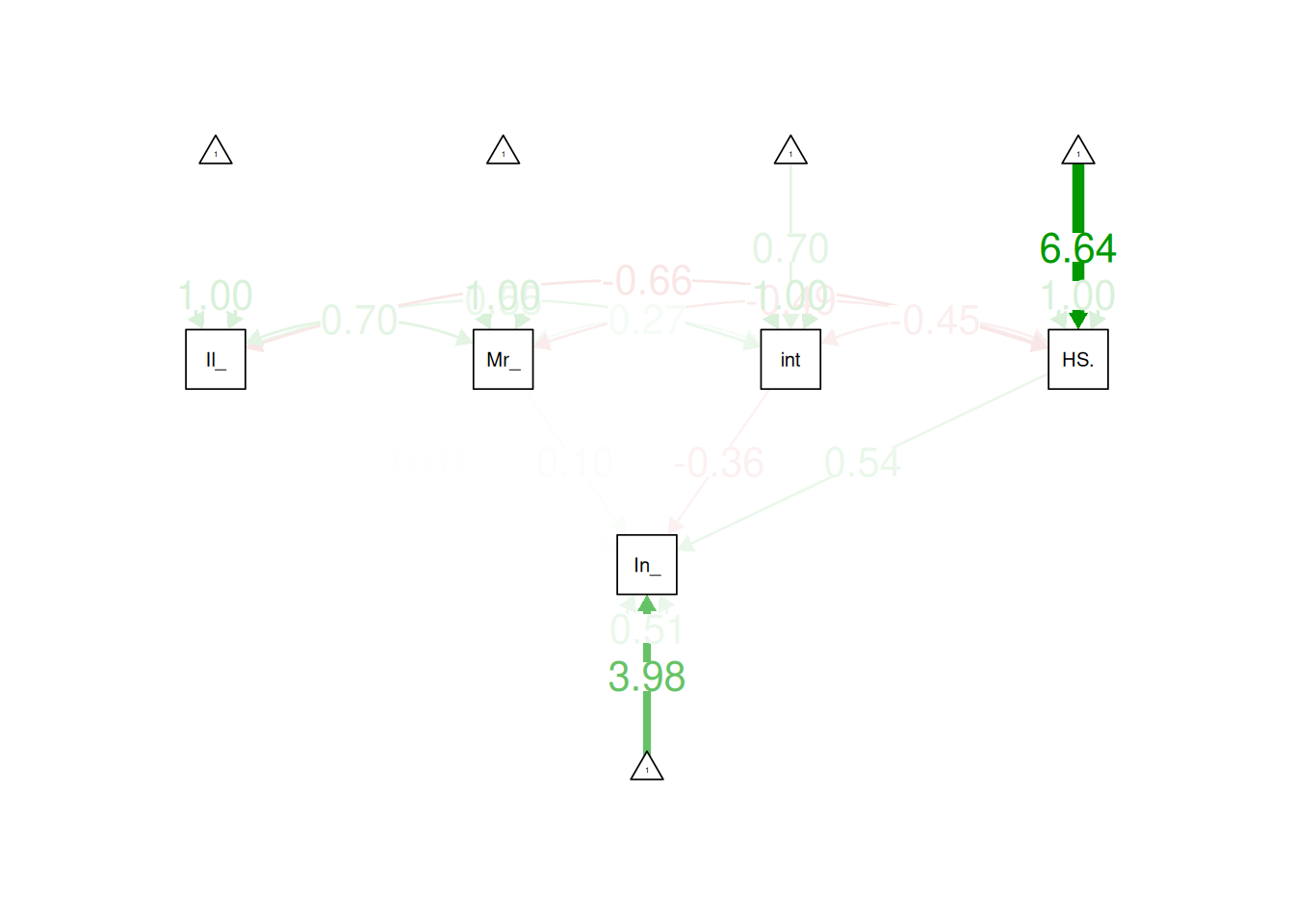
lavaanPlot::lavaanPlot(
moderationFit,
coefs = TRUE,
#covs = TRUE,
stand = TRUE)lavaanPlot::lavaanPlot2(
moderationFit,
#stand = TRUE, # currently throws error; uncomment out when fixed: https://github.com/alishinski/lavaanPlot/issues/52
coef_labels = TRUE)To generate an interactive/modifiable path diagram, you can use the following syntax:
lavaangui::plot_lavaan(moderationFit)# Created Model-Implied Predicted Data Object
modelImpliedPredictedData <- expand.grid(
Illiteracy_factor = c("Low","Middle","High"),
Murder_factor = c("Low","Middle","High"))
Illiteracy_mean <- mean(states$Illiteracy, na.rm = TRUE)
Illiteracy_sd <- sd(states$Illiteracy, na.rm = TRUE)
Murder_mean <- mean(states$Murder, na.rm = TRUE)
Murder_sd <- sd(states$Murder, na.rm = TRUE)
Illiteracy_centered_mean <- mean(states$Illiteracy_centered, na.rm = TRUE)
Illiteracy_centered_sd <- sd(states$Illiteracy_centered, na.rm = TRUE)
Murder_centered_mean <- mean(states$Murder_centered, na.rm = TRUE)
Murder_centered_sd <- sd(states$Murder_centered, na.rm = TRUE)
modelImpliedPredictedData <- modelImpliedPredictedData %>%
mutate(
Illiteracy = case_when(
Illiteracy_factor == "Low" ~ Illiteracy_mean - Illiteracy_sd,
Illiteracy_factor == "Middle" ~ Illiteracy_mean,
Illiteracy_factor == "High" ~ Illiteracy_mean + Illiteracy_sd
),
Illiteracy_centered = case_when(
Illiteracy_factor == "Low" ~ Illiteracy_centered_mean - Illiteracy_centered_sd,
Illiteracy_factor == "Middle" ~ Illiteracy_centered_mean,
Illiteracy_factor == "High" ~ Illiteracy_centered_mean + Illiteracy_centered_sd
),
Murder = case_when(
Murder_factor == "Low" ~ Murder_mean - Murder_sd,
Murder_factor == "Middle" ~ Murder_mean,
Murder_factor == "High" ~ Murder_mean + Murder_sd
),
Murder_centered = case_when(
Murder_factor == "Low" ~ Murder_centered_mean - Murder_centered_sd,
Murder_factor == "Middle" ~ Murder_centered_mean,
Murder_factor == "High" ~ Murder_centered_mean + Murder_centered_sd
),
interaction = Illiteracy_centered * Murder_centered,
HS.Grad = mean(states$HS.Grad, na.rm = TRUE), # mean for covariates
Income_rescaled = NA
)
Murder_labels <- factor(
modelImpliedPredictedData$Murder_factor,
levels = c("High", "Middle", "Low"),
labels = c("High (+1 SD)", "Middle (mean)", "Low (−1 SD)"))
modelImpliedPredictedData$Income_rescaled <- lavPredictY(
moderationFit,
newdata = modelImpliedPredictedData,
ynames = "Income_rescaled"
) %>%
as.vector()
# Verify Computation Manually
moderationFit_parameters <- parameterEstimates(moderationFit)
moderationFit_parametersintercept <- moderationFit_parameters[which(moderationFit_parameters$lhs == "Income_rescaled" & moderationFit_parameters$op == "~1"), "est"]
b_Illiteracy_centered <- moderationFit_parameters[which(moderationFit_parameters$lhs == "Income_rescaled" & moderationFit_parameters$rhs == "Illiteracy_centered"), "est"]
b_Murder_centered <- moderationFit_parameters[which(moderationFit_parameters$lhs == "Income_rescaled" & moderationFit_parameters$rhs == "Murder_centered"), "est"]
b_interaction <- moderationFit_parameters[which(moderationFit_parameters$lhs == "Income_rescaled" & moderationFit_parameters$rhs == "interaction"), "est"]
b_HS.Grad <- moderationFit_parameters[which(moderationFit_parameters$lhs == "Income_rescaled" & moderationFit_parameters$rhs == "HS.Grad"), "est"]
modelImpliedPredictedData <- modelImpliedPredictedData %>%
mutate(
Income_rescaled_calculatedManually = intercept + (b_Illiteracy_centered * Illiteracy_centered) + (b_Murder_centered * Murder_centered) + (b_interaction * interaction) + (b_HS.Grad * HS.Grad))
# Model-Implied Predicted Data
modelImpliedPredictedData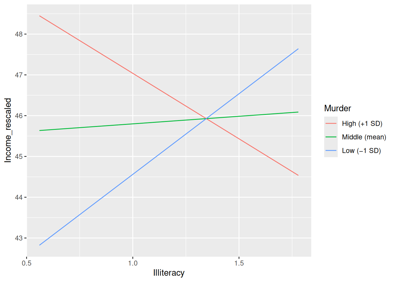
https://gabriellajg.github.io/EPSY-579-R-Cookbook-for-SEM/week6_1-lavaan-lab-4-mediated-moderation-moderated-mediation.html#step-5-johnson-neyman-interval (archived at https://perma.cc/6XR6-ZPSL)
# Find the min and max values of the moderator
Murder_centered_min <- min(modelImpliedPredictedData$Murder_centered, na.rm = TRUE)
Murder_centered_max <- max(modelImpliedPredictedData$Murder_centered, na.rm = TRUE)
Murder_centered_cutoff1 <- -1.5 # pick and titrate cutoff to help find the lower bound of the region of significance
Murder_centered_cutoff2 <- -1 # pick and titrate cutoff to help find the upper bound of the region of significance
Murder_centered_sd <- sd(modelImpliedPredictedData$Murder_centered, na.rm = TRUE)
Murder_centered_low <- mean(modelImpliedPredictedData$Murder_centered, na.rm = TRUE) - sd(modelImpliedPredictedData$Murder_centered, na.rm = TRUE)
Murder_centered_mean <- mean(modelImpliedPredictedData$Murder_centered, na.rm = TRUE)
Murder_centered_high <- mean(modelImpliedPredictedData$Murder_centered, na.rm = TRUE) + sd(modelImpliedPredictedData$Murder_centered, na.rm = TRUE)
# Extend the moderation model to compute the simple slopes and conditional effects at specific values of the moderator
moderationModelSimpleSlopes <- paste0('
# Regression
Income_rescaled ~ b1*Illiteracy_centered + b2*Murder_centered + b3*interaction + b4*HS.Grad
# Simple Slopes
SS_min := b1 + b3 * ', Murder_centered_min, '
SS_cutoff1 := b1 + b3 * ', Murder_centered_cutoff1, '
SS_cutoff2 := b1 + b3 * ', Murder_centered_cutoff2, '
SS_low := b1 + b3 * ', Murder_centered_low, '
SS_mean := b1 + b3 * ', Murder_centered_mean, '
SS_high := b1 + b3 * ', Murder_centered_high, '
SS_max := b1 + b3 * ', Murder_centered_max, '
')
# Fit the Model
set.seed(52242) # for reproducibility
moderationModelSimpleSlopes_fit <- sem(
model = moderationModelSimpleSlopes,
data = states,
missing = "ML",
estimator = "ML",
se = "bootstrap",
bootstrap = 1000,
std.lv = TRUE,
fixed.x = FALSE)
summary(
moderationModelSimpleSlopes_fit,
#fit.measures = TRUE,
standardized = TRUE,
rsquare = TRUE)lavaan 0.6-21 ended normally after 27 iterations
Estimator ML
Optimization method NLMINB
Number of model parameters 20
Number of observations 50
Number of missing patterns 1
Model Test User Model:
Test statistic 0.000
Degrees of freedom 0
Parameter Estimates:
Standard errors Bootstrap
Number of requested bootstrap draws 1000
Number of successful bootstrap draws 1000
Regressions:
Estimate Std.Err z-value P(>|z|) Std.lv Std.all
Income_rescaled ~
Illtrcy_c (b1) 0.371 2.266 0.164 0.870 0.371 0.037
Mrdr_cntr (b2) 0.171 0.271 0.630 0.528 0.171 0.103
interactn (b3) -0.970 0.307 -3.157 0.002 -0.970 -0.355
HS.Grad (b4) 0.408 0.162 2.521 0.012 0.408 0.536
Covariances:
Estimate Std.Err z-value P(>|z|) Std.lv Std.all
Illiteracy_centered ~~
Murder_centerd 1.550 0.312 4.963 0.000 1.550 0.703
interaction 0.733 0.320 2.290 0.022 0.733 0.546
HS.Grad -3.171 0.700 -4.532 0.000 -3.171 -0.657
Murder_centered ~~
interaction 2.223 1.596 1.393 0.164 2.223 0.273
HS.Grad -14.259 3.925 -3.633 0.000 -14.259 -0.488
interaction ~~
HS.Grad -7.938 2.988 -2.656 0.008 -7.938 -0.446
Intercepts:
Estimate Std.Err z-value P(>|z|) Std.lv Std.all
.Income_rescald 24.215 8.505 2.847 0.004 24.215 3.981
Illitrcy_cntrd -0.000 0.087 -0.000 1.000 -0.000 -0.000
Murder_centerd -0.000 0.524 -0.000 1.000 -0.000 -0.000
interaction 1.550 0.312 4.969 0.000 1.550 0.696
HS.Grad 53.108 1.124 47.235 0.000 53.108 6.642
Variances:
Estimate Std.Err z-value P(>|z|) Std.lv Std.all
.Income_rescald 19.006 3.928 4.838 0.000 19.006 0.514
Illitrcy_cntrd 0.364 0.065 5.586 0.000 0.364 1.000
Murder_centerd 13.355 1.780 7.501 0.000 13.355 1.000
interaction 4.956 1.441 3.439 0.001 4.956 1.000
HS.Grad 63.933 9.923 6.443 0.000 63.933 1.000
R-Square:
Estimate
Income_rescald 0.486
Defined Parameters:
Estimate Std.Err z-value P(>|z|) Std.lv Std.all
SS_min 3.953 2.924 1.352 0.176 3.953 1.348
SS_cutoff1 1.827 2.492 0.733 0.464 1.827 0.570
SS_cutoff2 1.342 2.409 0.557 0.578 1.342 0.392
SS_low 3.473 2.818 1.233 0.218 3.473 1.172
SS_mean 0.371 2.266 0.164 0.870 0.371 0.037
SS_high -2.731 2.063 -1.324 0.185 -2.731 -1.099
SS_max -3.211 2.071 -1.550 0.121 -3.211 -1.274moderationModelSimpleSlopesFit_parameters <- parameterEstimates(
moderationModelSimpleSlopes_fit,
level = 0.95,
boot.ci.type = "bca.simple")
moderationModelSimpleSlopesFit_parametersA simple slope of the predictor on the outcome is considered significant at a given level of the moderator if the 95% confidence interval from the bootstrapped estimates of the simple slopes at that level of the moderator (i.e., [ci.lower,ci.upper]) does not include zero. In this particular model, the predictor (Illiteracy) is not significant at any of the levels of the moderator (Murder), because the 95% confidence intervals of all simple slopes include zero, in this case, likely due to a small sample size (\(N = 50\)) and the resulting low power.
As I noted above, the predictor is not significant at any levels of the moderator. Nevertheless, I created a made up Johnson-Neyman plot by specifying the (fictitious) range of significance, for purposes of demonstration. The band around the line indicates the 95% confidence interval of the simple slope of the predictor on the outcome as a function of different levels of the moderator. In reality (unlike in this fictitious example), the regions of significance would only be regions where the 95% confidence interval of the simple slope does not include zero.
The standard error of the slope is the square root of the variance of the slope. The forumula for computing the standard error of the slope is based on the formula for computing the variance of a weighted sum.
The slope of the predictor on the outcome at different levels of the moderator is calculated as (Jaccard & Turisi, 2003):
\[ \text{slope}_\text{predictor} = b_1 + b_3 \cdot Z \]
The standard error of the slope of the predictor on the outcome at different levels of the moderator is calculated as (https://stats.stackexchange.com/a/55973/20338; archived at https://perma.cc/V255-853Z; Jaccard & Turisi, 2003):
\[ \begin{aligned} SE(\text{slope}_\text{predictor}) &= \sqrt{Var(b_1) + Var(b_3) \cdot Z^2 + 2 \cdot Z \cdot Cov(b_1, b_3)} \\ SE(b_1 + b_3 \cdot Z) &= \end{aligned} \]
where:
The variance of a weighted sum is:
\[ \begin{aligned} Var(\text{slope}_\text{predictor}) &= Var(b_1) + Var(b_3) \cdot Z^2 + 2 \cdot Z \cdot Cov(b_1, b_3) \\ Var(b_1 + b_3 \cdot Z) &= \end{aligned} \]
The standard error is the square root of the variance. The 95% confidence interval of the slope is \(\pm\) 1.959964 (i.e., qnorm(.975)) standard errors of the slope estimate.
# Create a data frame for plotting
Murder_min <- min(states$Murder, na.rm = TRUE)
Murder_max <- max(states$Murder, na.rm = TRUE)
plot_data <- data.frame(
Murder = seq(Murder_min, Murder_max, length.out = 10000)
)
plot_data$Murder_centered <- scale(plot_data$Murder, scale = FALSE)
# Calculate predicted slopes and confidence intervals
b1 <- moderationModelSimpleSlopesFit_parameters[which(moderationModelSimpleSlopesFit_parameters$label == "b1"), "est"]
b3 <- moderationModelSimpleSlopesFit_parameters[which(moderationModelSimpleSlopesFit_parameters$label == "b3"), "est"]
b1_se <- moderationModelSimpleSlopesFit_parameters[which(moderationModelSimpleSlopesFit_parameters$label == "b1"), "se"]
b3_se <- moderationModelSimpleSlopesFit_parameters[which(moderationModelSimpleSlopesFit_parameters$label == "b3"), "se"]
varianceCovarianceMatrix <- vcov(moderationFit)
b1_var <- varianceCovarianceMatrix["Income_rescaled~Illiteracy_centered","Income_rescaled~Illiteracy_centered"]
b3_var <- varianceCovarianceMatrix["interaction~~interaction","interaction~~interaction"]
cov_b1b3 <- varianceCovarianceMatrix["Income_rescaled~Illiteracy_centered","interaction~~interaction"]
#sqrt((b1_se^2) + ((b3_se^2) * plot_data$Murder_centered^2) + (2 * plot_data$Murder_centered * cov_b1b3))
#sqrt((b1_var) + ((b3_var) * plot_data$Murder_centered^2) + (2 * plot_data$Murder_centered * cov_b1b3))
plot_data$predicted_slopes <- b1 + b3 * plot_data$Murder_centered
plot_data$slope_se <- sqrt((b1_var) + ((b3_var) * plot_data$Murder_centered^2) + (2 * plot_data$Murder_centered * cov_b1b3))
# Calculated the 95% confidence interval around the simple slope
plot_data$lower_ci <- plot_data$predicted_slopes - qnorm(.975) * plot_data$slope_se
plot_data$upper_ci <- plot_data$predicted_slopes + qnorm(.975) * plot_data$slope_se
# Specify the significant range (based on the regions identified in the simple slopes analysis, see "Simple Slopes and Regions of Significance" section above)
plot_data$significant_slope <- FALSE
plot_data$significant_slope[which(plot_data$Murder_centered < -4.2 | plot_data$Murder_centered > 3.75)] <-TRUE # specify significant range
# Specify the significant region number (there are either 0, 1, or 2 significant regions; in such cases, there would be 1, 0 or 1 or 2, or 1 nonsignificant regions, respectively)--for instance, sig from 0-4, ns from 4-12, and sig from 12-16 would be 2 significant regions and 1 nonsignificant region
plot_data$significantRegionNumber <- NA
plot_data$significantRegionNumber[which(plot_data$Murder_centered < -4.2)] <- 1 # specify significant range 1
plot_data$significantRegionNumber[which(plot_data$Murder_centered > 3.75)] <- 2 # specify significant range 2
min(plot_data$Murder[which(plot_data$significant_slope == FALSE)])[1] 4.051215[1] 11.99938ggplot(plot_data, aes(x = Murder, y = predicted_slopes)) +
geom_ribbon(
data = plot_data %>% filter(significant_slope == FALSE),
aes(ymin = lower_ci, ymax = upper_ci),
fill = "#F8766D",
alpha = 0.2) +
geom_ribbon(
data = plot_data %>% filter(significantRegionNumber == 1),
aes(ymin = lower_ci, ymax = upper_ci),
fill = "#00BFC4",
alpha = 0.2) +
geom_ribbon(
data = plot_data %>% filter(significantRegionNumber == 2),
aes(ymin = lower_ci, ymax = upper_ci),
fill = "#00BFC4",
alpha = 0.2) +
geom_line(
data = plot_data %>% filter(significant_slope == FALSE),
aes(x = Murder, y = predicted_slopes),
color = "#F8766D",
linewidth = 2) +
geom_line(
data = plot_data %>% filter(significantRegionNumber == 1),
aes(x = Murder, y = predicted_slopes),
color = "#00BFC4",
linewidth = 2) +
geom_line(
data = plot_data %>% filter(significantRegionNumber == 2),
aes(x = Murder, y = predicted_slopes),
color = "#00BFC4",
linewidth = 2) +
geom_hline(yintercept = 0, linetype = "dashed") +
geom_vline(xintercept = c(4.051215, 11.99938), linetype = 2, color = "#00BFC4") + # update based on numbers above
labs(
title = "Johnson-Neyman Plot",
subtitle = "(blue = significant slope; pink = nonsignificant slope)",
x = "Moderator (Murder)",
y = "Simple Slope of Predictor (Illiteracy)") +
theme_classic()
There are several options for examining latent variable moderation/interaction:
modsem package and Mplus)semTools package)The code examples below follow the approach suggested by Widaman et al. (2010).
Widaman, K. F., Ferrer, E., & Conger, R. D. (2010). Factorial invariance within longitudinal structural equation models: Measuring the same construct across time. Child Development Perspectives, 4(1), 10–18. https://doi.org/10.1111/j.1750-8606.2009.00110.x
For the longitudinal measurement invariance models, we use simulated data from https://mycourses.aalto.fi/mod/assign/view.php?id=1203047 (archived at https://perma.cc/QTL2-ZHX2). As noted here (archived at https://perma.cc/QTL2-ZHX2), “The data are in wide format where the variables are coded as [VARIABLE NAME][time index][indicator index].”
Evaluates whether there are the same number of latent factors across time and whether the indicators load onto the same latent factor(s) across time.
configuralInvariance_syntax <- '
# Factor Loadings
jobsat_1 =~ NA*loadj1*JOBSAT11 + JOBSAT12 + JOBSAT13
jobsat_2 =~ NA*loadj1*JOBSAT21 + JOBSAT22 + JOBSAT23
jobsat_3 =~ NA*loadj1*JOBSAT31 + JOBSAT32 + JOBSAT33
ready_1 =~ NA*loadr1*READY11 + READY12 + READY13
ready_2 =~ NA*loadr1*READY21 + READY22 + READY23
ready_3 =~ NA*loadr1*READY31 + READY32 + READY33
commit_1 =~ NA*loadc1*COMMIT11 + COMMIT12 + COMMIT13
commit_2 =~ NA*loadc1*COMMIT21 + COMMIT22 + COMMIT23
commit_3 =~ NA*loadc1*COMMIT31 + COMMIT32 + COMMIT33
# Factor Identification: Standardize Factors at T1
## Fix Factor Means at T1 to Zero
jobsat_1 ~ 0*1
ready_1 ~ 0*1
commit_1 ~ 0*1
## Fix Factor Variances at T1 to One
jobsat_1 ~~ 1*jobsat_1
ready_1 ~~ 1*ready_1
commit_1 ~~ 1*commit_1
# Freely Estimate Factor Means at T2 and T3 (relative to T1)
jobsat_2 ~ 1
jobsat_3 ~ 1
ready_2 ~ 1
ready_3 ~ 1
commit_2 ~ 1
commit_3 ~ 1
# Freely Estimate Factor Variances at T2 and T3 (relative to T1)
jobsat_2 ~~ jobsat_2
jobsat_3 ~~ jobsat_3
ready_2 ~~ ready_2
ready_3 ~~ ready_3
commit_2 ~~ commit_2
commit_3 ~~ commit_3
# Fix Intercepts of Indicator 1 Across Time
JOBSAT11 ~ intj1*1
JOBSAT21 ~ intj1*1
JOBSAT31 ~ intj1*1
READY11 ~ intr1*1
READY21 ~ intr1*1
READY31 ~ intr1*1
COMMIT11 ~ intc1*1
COMMIT21 ~ intc1*1
COMMIT31 ~ intc1*1
# Free Intercepts of Remaining Manifest Variables
JOBSAT12 ~ 1
JOBSAT13 ~ 1
JOBSAT22 ~ 1
JOBSAT23 ~ 1
JOBSAT32 ~ 1
JOBSAT33 ~ 1
READY12 ~ 1
READY13 ~ 1
READY22 ~ 1
READY23 ~ 1
READY32 ~ 1
READY33 ~ 1
COMMIT12 ~ 1
COMMIT13 ~ 1
COMMIT22 ~ 1
COMMIT23 ~ 1
COMMIT32 ~ 1
COMMIT33 ~ 1
# Estimate Residual Variances of Manifest Variables
JOBSAT11 ~~ JOBSAT11
JOBSAT12 ~~ JOBSAT12
JOBSAT13 ~~ JOBSAT13
JOBSAT21 ~~ JOBSAT21
JOBSAT22 ~~ JOBSAT22
JOBSAT23 ~~ JOBSAT23
JOBSAT31 ~~ JOBSAT31
JOBSAT32 ~~ JOBSAT32
JOBSAT33 ~~ JOBSAT33
READY11 ~~ READY11
READY12 ~~ READY12
READY13 ~~ READY13
READY21 ~~ READY21
READY22 ~~ READY22
READY23 ~~ READY23
READY31 ~~ READY31
READY32 ~~ READY32
READY33 ~~ READY33
COMMIT11 ~~ COMMIT11
COMMIT12 ~~ COMMIT12
COMMIT13 ~~ COMMIT13
COMMIT21 ~~ COMMIT21
COMMIT22 ~~ COMMIT22
COMMIT23 ~~ COMMIT23
COMMIT31 ~~ COMMIT31
COMMIT32 ~~ COMMIT32
COMMIT33 ~~ COMMIT33
'configuralInvariance_fit <- cfa(
configuralInvariance_syntax,
data = longitudinalMI,
missing = "ML",
estimator = "MLR",
meanstructure = TRUE,
#std.lv = TRUE,
fixed.x = FALSE)summary(
configuralInvariance_fit,
fit.measures = TRUE,
standardized = TRUE,
rsquare = TRUE)lavaan 0.6-21 ended normally after 101 iterations
Estimator ML
Optimization method NLMINB
Number of model parameters 129
Number of equality constraints 12
Number of observations 495
Number of missing patterns 1
Model Test User Model:
Standard Scaled
Test Statistic 770.816 783.291
Degrees of freedom 288 288
P-value (Chi-square) 0.000 0.000
Scaling correction factor 0.984
Yuan-Bentler correction (Mplus variant)
Model Test Baseline Model:
Test statistic 6697.063 6541.933
Degrees of freedom 351 351
P-value 0.000 0.000
Scaling correction factor 1.024
User Model versus Baseline Model:
Comparative Fit Index (CFI) 0.924 0.920
Tucker-Lewis Index (TLI) 0.907 0.902
Robust Comparative Fit Index (CFI) 0.923
Robust Tucker-Lewis Index (TLI) 0.906
Loglikelihood and Information Criteria:
Loglikelihood user model (H0) -17716.771 -17716.771
Scaling correction factor 0.935
for the MLR correction
Loglikelihood unrestricted model (H1) -17331.363 -17331.363
Scaling correction factor 0.998
for the MLR correction
Akaike (AIC) 35667.543 35667.543
Bayesian (BIC) 36159.476 36159.476
Sample-size adjusted Bayesian (SABIC) 35788.115 35788.115
Root Mean Square Error of Approximation:
RMSEA 0.058 0.059
90 Percent confidence interval - lower 0.053 0.054
90 Percent confidence interval - upper 0.063 0.064
P-value H_0: RMSEA <= 0.050 0.003 0.002
P-value H_0: RMSEA >= 0.080 0.000 0.000
Robust RMSEA 0.058
90 Percent confidence interval - lower 0.054
90 Percent confidence interval - upper 0.063
P-value H_0: Robust RMSEA <= 0.050 0.002
P-value H_0: Robust RMSEA >= 0.080 0.000
Standardized Root Mean Square Residual:
SRMR 0.032 0.032
Parameter Estimates:
Standard errors Sandwich
Information bread Observed
Observed information based on Hessian
Latent Variables:
Estimate Std.Err z-value P(>|z|) Std.lv Std.all
jobsat_1 =~
JOBSAT1 (ldj1) 0.996 0.041 24.099 0.000 0.996 0.818
JOBSAT1 1.019 0.042 24.487 0.000 1.019 0.814
JOBSAT1 0.956 0.040 23.787 0.000 0.956 0.798
jobsat_2 =~
JOBSAT2 (ldj1) 0.996 0.041 24.099 0.000 0.961 0.796
JOBSAT2 1.001 0.058 17.194 0.000 0.967 0.805
JOBSAT2 0.964 0.064 15.021 0.000 0.931 0.785
jobsat_3 =~
JOBSAT3 (ldj1) 0.996 0.041 24.099 0.000 0.861 0.776
JOBSAT3 0.980 0.066 14.839 0.000 0.848 0.773
JOBSAT3 1.070 0.071 15.159 0.000 0.926 0.806
ready_1 =~
READY11 (ldr1) 0.900 0.042 21.255 0.000 0.900 0.781
READY12 0.882 0.043 20.311 0.000 0.882 0.766
READY13 0.905 0.041 21.860 0.000 0.905 0.789
ready_2 =~
READY21 (ldr1) 0.900 0.042 21.255 0.000 0.947 0.795
READY22 0.785 0.053 14.924 0.000 0.826 0.731
READY23 0.821 0.056 14.581 0.000 0.864 0.750
ready_3 =~
READY31 (ldr1) 0.900 0.042 21.255 0.000 0.878 0.764
READY32 0.847 0.062 13.766 0.000 0.827 0.750
READY33 0.888 0.070 12.759 0.000 0.867 0.757
commit_1 =~
COMMIT1 (ldc1) 0.809 0.044 18.389 0.000 0.809 0.748
COMMIT1 0.825 0.041 19.985 0.000 0.825 0.755
COMMIT1 0.815 0.042 19.477 0.000 0.815 0.753
commit_2 =~
COMMIT2 (ldc1) 0.809 0.044 18.389 0.000 0.854 0.768
COMMIT2 0.818 0.058 14.105 0.000 0.863 0.768
COMMIT2 0.866 0.062 13.866 0.000 0.914 0.787
commit_3 =~
COMMIT3 (ldc1) 0.809 0.044 18.389 0.000 0.774 0.752
COMMIT3 0.771 0.059 13.123 0.000 0.738 0.706
COMMIT3 0.812 0.066 12.398 0.000 0.777 0.728
Covariances:
Estimate Std.Err z-value P(>|z|) Std.lv Std.all
jobsat_1 ~~
jobsat_2 0.436 0.058 7.532 0.000 0.451 0.451
jobsat_3 0.325 0.052 6.288 0.000 0.375 0.375
ready_1 0.542 0.050 10.840 0.000 0.542 0.542
ready_2 0.286 0.062 4.611 0.000 0.271 0.271
ready_3 0.176 0.057 3.105 0.002 0.181 0.181
commit_1 0.581 0.046 12.496 0.000 0.581 0.581
commit_2 0.380 0.063 6.086 0.000 0.360 0.360
commit_3 0.237 0.056 4.211 0.000 0.248 0.248
jobsat_2 ~~
jobsat_3 0.381 0.057 6.665 0.000 0.456 0.456
ready_1 0.198 0.057 3.494 0.000 0.205 0.205
ready_2 0.508 0.067 7.574 0.000 0.500 0.500
ready_3 0.193 0.057 3.405 0.001 0.205 0.205
commit_1 0.278 0.055 5.049 0.000 0.288 0.288
commit_2 0.584 0.070 8.297 0.000 0.573 0.573
commit_3 0.260 0.059 4.431 0.000 0.281 0.281
jobsat_3 ~~
ready_1 0.201 0.048 4.224 0.000 0.232 0.232
ready_2 0.272 0.054 5.051 0.000 0.298 0.298
ready_3 0.451 0.063 7.182 0.000 0.534 0.534
commit_1 0.182 0.052 3.489 0.000 0.210 0.210
commit_2 0.265 0.059 4.503 0.000 0.290 0.290
commit_3 0.480 0.061 7.885 0.000 0.580 0.580
ready_1 ~~
ready_2 0.404 0.066 6.073 0.000 0.383 0.383
ready_3 0.323 0.059 5.445 0.000 0.331 0.331
commit_1 0.452 0.050 9.057 0.000 0.452 0.452
commit_2 0.282 0.065 4.332 0.000 0.267 0.267
commit_3 0.230 0.058 3.990 0.000 0.240 0.240
ready_2 ~~
ready_3 0.515 0.077 6.723 0.000 0.501 0.501
commit_1 0.270 0.062 4.373 0.000 0.256 0.256
commit_2 0.694 0.086 8.052 0.000 0.625 0.625
commit_3 0.309 0.066 4.709 0.000 0.307 0.307
ready_3 ~~
commit_1 0.175 0.059 2.981 0.003 0.180 0.180
commit_2 0.298 0.067 4.478 0.000 0.289 0.289
commit_3 0.452 0.070 6.414 0.000 0.484 0.484
commit_1 ~~
commit_2 0.632 0.065 9.669 0.000 0.598 0.598
commit_3 0.427 0.059 7.214 0.000 0.447 0.447
commit_2 ~~
commit_3 0.583 0.090 6.510 0.000 0.577 0.577
Intercepts:
Estimate Std.Err z-value P(>|z|) Std.lv Std.all
jbst_1 0.000 0.000 0.000
redy_1 0.000 0.000 0.000
cmmt_1 0.000 0.000 0.000
jbst_2 -0.000 0.062 -0.000 1.000 -0.000 -0.000
jbst_3 0.126 0.060 2.099 0.036 0.145 0.145
redy_2 0.056 0.070 0.802 0.422 0.053 0.053
redy_3 0.204 0.073 2.818 0.005 0.209 0.209
cmmt_2 -0.200 0.069 -2.885 0.004 -0.189 -0.189
cmmt_3 -0.172 0.071 -2.442 0.015 -0.180 -0.180
.JOBSAT (intj1) 3.319 0.055 60.662 0.000 3.319 2.727
.JOBSAT (intj1) 3.319 0.055 60.662 0.000 3.319 2.749
.JOBSAT (intj1) 3.319 0.055 60.662 0.000 3.319 2.989
.READY1 (intr1) 3.176 0.052 61.297 0.000 3.176 2.755
.READY2 (intr1) 3.176 0.052 61.297 0.000 3.176 2.665
.READY3 (intr1) 3.176 0.052 61.297 0.000 3.176 2.763
.COMMIT (intc1) 3.719 0.049 76.578 0.000 3.719 3.442
.COMMIT (intc1) 3.719 0.049 76.578 0.000 3.719 3.345
.COMMIT (intc1) 3.719 0.049 76.578 0.000 3.719 3.613
.JOBSAT 3.311 0.056 58.833 0.000 3.311 2.644
.JOBSAT 3.321 0.054 61.701 0.000 3.321 2.773
.JOBSAT 3.331 0.067 49.733 0.000 3.331 2.774
.JOBSAT 3.329 0.067 49.620 0.000 3.329 2.805
.JOBSAT 3.281 0.065 50.616 0.000 3.281 2.992
.JOBSAT 3.251 0.070 46.441 0.000 3.251 2.830
.READY1 3.198 0.052 61.778 0.000 3.198 2.777
.READY1 3.156 0.052 61.219 0.000 3.156 2.752
.READY2 3.170 0.061 51.554 0.000 3.170 2.807
.READY2 3.211 0.062 51.499 0.000 3.211 2.788
.READY3 3.156 0.066 47.871 0.000 3.156 2.864
.READY3 3.146 0.070 44.635 0.000 3.146 2.747
.COMMIT 3.653 0.049 74.420 0.000 3.653 3.345
.COMMIT 3.596 0.049 73.962 0.000 3.596 3.324
.COMMIT 3.689 0.064 57.387 0.000 3.689 3.282
.COMMIT 3.662 0.066 55.846 0.000 3.662 3.153
.COMMIT 3.749 0.061 61.081 0.000 3.749 3.586
.COMMIT 3.692 0.064 57.657 0.000 3.692 3.457
Variances:
Estimate Std.Err z-value P(>|z|) Std.lv Std.all
jobsat_1 1.000 1.000 1.000
ready_1 1.000 1.000 1.000
commit_1 1.000 1.000 1.000
jobsat_2 0.933 0.098 9.534 0.000 1.000 1.000
jobsat_3 0.748 0.087 8.650 0.000 1.000 1.000
ready_2 1.108 0.122 9.097 0.000 1.000 1.000
ready_3 0.952 0.122 7.786 0.000 1.000 1.000
commit_2 1.114 0.146 7.615 0.000 1.000 1.000
commit_3 0.916 0.127 7.204 0.000 1.000 1.000
.JOBSAT11 0.491 0.051 9.630 0.000 0.491 0.331
.JOBSAT12 0.529 0.049 10.895 0.000 0.529 0.337
.JOBSAT13 0.521 0.046 11.315 0.000 0.521 0.363
.JOBSAT21 0.533 0.052 10.209 0.000 0.533 0.366
.JOBSAT22 0.506 0.047 10.685 0.000 0.506 0.351
.JOBSAT23 0.542 0.052 10.394 0.000 0.542 0.384
.JOBSAT31 0.491 0.042 11.704 0.000 0.491 0.398
.JOBSAT32 0.484 0.043 11.164 0.000 0.484 0.403
.JOBSAT33 0.463 0.046 10.128 0.000 0.463 0.350
.READY11 0.519 0.051 10.112 0.000 0.519 0.391
.READY12 0.548 0.048 11.392 0.000 0.548 0.413
.READY13 0.496 0.048 10.318 0.000 0.496 0.377
.READY21 0.522 0.054 9.742 0.000 0.522 0.368
.READY22 0.593 0.049 12.067 0.000 0.593 0.465
.READY23 0.580 0.055 10.611 0.000 0.580 0.437
.READY31 0.550 0.054 10.190 0.000 0.550 0.417
.READY32 0.531 0.048 11.179 0.000 0.531 0.437
.READY33 0.560 0.048 11.585 0.000 0.560 0.427
.COMMIT11 0.514 0.050 10.191 0.000 0.514 0.440
.COMMIT12 0.512 0.045 11.266 0.000 0.512 0.429
.COMMIT13 0.506 0.047 10.756 0.000 0.506 0.432
.COMMIT21 0.508 0.046 10.932 0.000 0.508 0.411
.COMMIT22 0.518 0.047 11.112 0.000 0.518 0.410
.COMMIT23 0.513 0.051 10.121 0.000 0.513 0.380
.COMMIT31 0.461 0.043 10.761 0.000 0.461 0.435
.COMMIT32 0.548 0.054 10.095 0.000 0.548 0.501
.COMMIT33 0.536 0.048 11.080 0.000 0.536 0.470
R-Square:
Estimate
JOBSAT11 0.669
JOBSAT12 0.663
JOBSAT13 0.637
JOBSAT21 0.634
JOBSAT22 0.649
JOBSAT23 0.616
JOBSAT31 0.602
JOBSAT32 0.597
JOBSAT33 0.650
READY11 0.609
READY12 0.587
READY13 0.623
READY21 0.632
READY22 0.535
READY23 0.563
READY31 0.583
READY32 0.563
READY33 0.573
COMMIT11 0.560
COMMIT12 0.571
COMMIT13 0.568
COMMIT21 0.589
COMMIT22 0.590
COMMIT23 0.620
COMMIT31 0.565
COMMIT32 0.499
COMMIT33 0.530modificationindices(
configuralInvariance_fit,
sort. = TRUE)lavaanPlot::lavaanPlot2(
configuralInvariance_fit,
stand = TRUE,
coef_labels = TRUE)Path Diagram
To generate an interactive/modifiable path diagram, you can use the following syntax:
lavaangui::plot_lavaan(configuralInvariance_fit)Evaluates whether the items’ factor loadings are the same across time.
metricInvariance_syntax <- '
# Factor Loadings
jobsat_1 =~ NA*loadj1*JOBSAT11 + loadj2*JOBSAT12 + loadj3*JOBSAT13
jobsat_2 =~ NA*loadj1*JOBSAT21 + loadj2*JOBSAT22 + loadj3*JOBSAT23
jobsat_3 =~ NA*loadj1*JOBSAT31 + loadj2*JOBSAT32 + loadj3*JOBSAT33
ready_1 =~ NA*loadr1*READY11 + loadr2*READY12 + loadr3*READY13
ready_2 =~ NA*loadr1*READY21 + loadr2*READY22 + loadr3*READY23
ready_3 =~ NA*loadr1*READY31 + loadr2*READY32 + loadr3*READY33
commit_1 =~ NA*loadc1*COMMIT11 + loadc2*COMMIT12 + loadc3*COMMIT13
commit_2 =~ NA*loadc1*COMMIT21 + loadc2*COMMIT22 + loadc3*COMMIT23
commit_3 =~ NA*loadc1*COMMIT31 + loadc2*COMMIT32 + loadc3*COMMIT33
# Factor Identification: Standardize Factors at T1
## Fix Factor Means at T1 to Zero
jobsat_1 ~ 0*1
ready_1 ~ 0*1
commit_1 ~ 0*1
## Fix Factor Variances at T1 to One
jobsat_1 ~~ 1*jobsat_1
ready_1 ~~ 1*ready_1
commit_1 ~~ 1*commit_1
# Freely Estimate Factor Means at T2 and T3 (relative to T1)
jobsat_2 ~ 1
jobsat_3 ~ 1
ready_2 ~ 1
ready_3 ~ 1
commit_2 ~ 1
commit_3 ~ 1
# Freely Estimate Factor Variances at T2 and T3 (relative to T1)
jobsat_2 ~~ jobsat_2
jobsat_3 ~~ jobsat_3
ready_2 ~~ ready_2
ready_3 ~~ ready_3
commit_2 ~~ commit_2
commit_3 ~~ commit_3
# Fix Intercepts of Indicator 1 Across Time
JOBSAT11 ~ intj1*1
JOBSAT21 ~ intj1*1
JOBSAT31 ~ intj1*1
READY11 ~ intr1*1
READY21 ~ intr1*1
READY31 ~ intr1*1
COMMIT11 ~ intc1*1
COMMIT21 ~ intc1*1
COMMIT31 ~ intc1*1
# Free Intercepts of Remaining Manifest Variables
JOBSAT12 ~ 1
JOBSAT13 ~ 1
JOBSAT22 ~ 1
JOBSAT23 ~ 1
JOBSAT32 ~ 1
JOBSAT33 ~ 1
READY12 ~ 1
READY13 ~ 1
READY22 ~ 1
READY23 ~ 1
READY32 ~ 1
READY33 ~ 1
COMMIT12 ~ 1
COMMIT13 ~ 1
COMMIT22 ~ 1
COMMIT23 ~ 1
COMMIT32 ~ 1
COMMIT33 ~ 1
# Estimate Residual Variances of Manifest Variables
JOBSAT11 ~~ JOBSAT11
JOBSAT12 ~~ JOBSAT12
JOBSAT13 ~~ JOBSAT13
JOBSAT21 ~~ JOBSAT21
JOBSAT22 ~~ JOBSAT22
JOBSAT23 ~~ JOBSAT23
JOBSAT31 ~~ JOBSAT31
JOBSAT32 ~~ JOBSAT32
JOBSAT33 ~~ JOBSAT33
READY11 ~~ READY11
READY12 ~~ READY12
READY13 ~~ READY13
READY21 ~~ READY21
READY22 ~~ READY22
READY23 ~~ READY23
READY31 ~~ READY31
READY32 ~~ READY32
READY33 ~~ READY33
COMMIT11 ~~ COMMIT11
COMMIT12 ~~ COMMIT12
COMMIT13 ~~ COMMIT13
COMMIT21 ~~ COMMIT21
COMMIT22 ~~ COMMIT22
COMMIT23 ~~ COMMIT23
COMMIT31 ~~ COMMIT31
COMMIT32 ~~ COMMIT32
COMMIT33 ~~ COMMIT33
# Residual Covariances Within Indicator Across Time
JOBSAT11 ~~ JOBSAT21
JOBSAT21 ~~ JOBSAT31
JOBSAT11 ~~ JOBSAT31
JOBSAT12 ~~ JOBSAT22
JOBSAT22 ~~ JOBSAT32
JOBSAT12 ~~ JOBSAT32
JOBSAT13 ~~ JOBSAT23
JOBSAT23 ~~ JOBSAT33
JOBSAT13 ~~ JOBSAT33
READY11 ~~ READY21
READY21 ~~ READY31
READY11 ~~ READY31
READY12 ~~ READY22
READY22 ~~ READY32
READY12 ~~ READY32
READY13 ~~ READY23
READY23 ~~ READY33
READY13 ~~ READY33
COMMIT11 ~~ COMMIT21
COMMIT21 ~~ COMMIT31
COMMIT11 ~~ COMMIT31
COMMIT12 ~~ COMMIT22
COMMIT22 ~~ COMMIT32
COMMIT12 ~~ COMMIT32
COMMIT13 ~~ COMMIT23
COMMIT23 ~~ COMMIT33
COMMIT13 ~~ COMMIT33
'metricInvariance_fit <- cfa(
metricInvariance_syntax,
data = longitudinalMI,
missing = "ML",
estimator = "MLR",
meanstructure = TRUE,
#std.lv = TRUE,
fixed.x = FALSE)summary(
metricInvariance_fit,
fit.measures = TRUE,
standardized = TRUE,
rsquare = TRUE)lavaan 0.6-21 ended normally after 91 iterations
Estimator ML
Optimization method NLMINB
Number of model parameters 156
Number of equality constraints 24
Number of observations 495
Number of missing patterns 1
Model Test User Model:
Standard Scaled
Test Statistic 286.159 292.814
Degrees of freedom 273 273
P-value (Chi-square) 0.280 0.196
Scaling correction factor 0.977
Yuan-Bentler correction (Mplus variant)
Model Test Baseline Model:
Test statistic 6697.063 6541.933
Degrees of freedom 351 351
P-value 0.000 0.000
Scaling correction factor 1.024
User Model versus Baseline Model:
Comparative Fit Index (CFI) 0.998 0.997
Tucker-Lewis Index (TLI) 0.997 0.996
Robust Comparative Fit Index (CFI) 0.997
Robust Tucker-Lewis Index (TLI) 0.996
Loglikelihood and Information Criteria:
Loglikelihood user model (H0) -17474.443 -17474.443
Scaling correction factor 0.880
for the MLR correction
Loglikelihood unrestricted model (H1) -17331.363 -17331.363
Scaling correction factor 0.998
for the MLR correction
Akaike (AIC) 35212.885 35212.885
Bayesian (BIC) 35767.887 35767.887
Sample-size adjusted Bayesian (SABIC) 35348.916 35348.916
Root Mean Square Error of Approximation:
RMSEA 0.010 0.012
90 Percent confidence interval - lower 0.000 0.000
90 Percent confidence interval - upper 0.021 0.022
P-value H_0: RMSEA <= 0.050 1.000 1.000
P-value H_0: RMSEA >= 0.080 0.000 0.000
Robust RMSEA 0.012
90 Percent confidence interval - lower 0.000
90 Percent confidence interval - upper 0.022
P-value H_0: Robust RMSEA <= 0.050 1.000
P-value H_0: Robust RMSEA >= 0.080 0.000
Standardized Root Mean Square Residual:
SRMR 0.024 0.024
Parameter Estimates:
Standard errors Sandwich
Information bread Observed
Observed information based on Hessian
Latent Variables:
Estimate Std.Err z-value P(>|z|) Std.lv Std.all
jobsat_1 =~
JOBSAT1 (ldj1) 0.974 0.036 26.751 0.000 0.974 0.807
JOBSAT1 (ldj2) 0.995 0.035 28.661 0.000 0.995 0.801
JOBSAT1 (ldj3) 0.995 0.036 27.941 0.000 0.995 0.819
jobsat_2 =~
JOBSAT2 (ldj1) 0.974 0.036 26.751 0.000 0.937 0.781
JOBSAT2 (ldj2) 0.995 0.035 28.661 0.000 0.957 0.803
JOBSAT2 (ldj3) 0.995 0.036 27.941 0.000 0.957 0.797
jobsat_3 =~
JOBSAT3 (ldj1) 0.974 0.036 26.751 0.000 0.866 0.778
JOBSAT3 (ldj2) 0.995 0.035 28.661 0.000 0.884 0.793
JOBSAT3 (ldj3) 0.995 0.036 27.941 0.000 0.884 0.783
ready_1 =~
READY11 (ldr1) 0.930 0.036 25.486 0.000 0.930 0.797
READY12 (ldr2) 0.850 0.036 23.877 0.000 0.850 0.748
READY13 (ldr3) 0.899 0.036 24.965 0.000 0.899 0.785
ready_2 =~
READY21 (ldr1) 0.930 0.036 25.486 0.000 0.916 0.779
READY22 (ldr2) 0.850 0.036 23.877 0.000 0.837 0.737
READY23 (ldr3) 0.899 0.036 24.965 0.000 0.886 0.763
ready_3 =~
READY31 (ldr1) 0.930 0.036 25.486 0.000 0.893 0.773
READY32 (ldr2) 0.850 0.036 23.877 0.000 0.816 0.743
READY33 (ldr3) 0.899 0.036 24.965 0.000 0.864 0.756
commit_1 =~
COMMIT1 (ldc1) 0.807 0.036 22.195 0.000 0.807 0.749
COMMIT1 (ldc2) 0.807 0.036 22.194 0.000 0.807 0.744
COMMIT1 (ldc3) 0.826 0.036 22.787 0.000 0.826 0.759
commit_2 =~
COMMIT2 (ldc1) 0.807 0.036 22.195 0.000 0.870 0.778
COMMIT2 (ldc2) 0.807 0.036 22.194 0.000 0.870 0.773
COMMIT2 (ldc3) 0.826 0.036 22.787 0.000 0.891 0.773
commit_3 =~
COMMIT3 (ldc1) 0.807 0.036 22.195 0.000 0.758 0.741
COMMIT3 (ldc2) 0.807 0.036 22.194 0.000 0.758 0.720
COMMIT3 (ldc3) 0.826 0.036 22.787 0.000 0.776 0.727
Covariances:
Estimate Std.Err z-value P(>|z|) Std.lv Std.all
.JOBSAT11 ~~
.JOBSAT21 0.118 0.032 3.655 0.000 0.118 0.222
.JOBSAT21 ~~
.JOBSAT31 0.123 0.032 3.905 0.000 0.123 0.235
.JOBSAT11 ~~
.JOBSAT31 0.151 0.029 5.126 0.000 0.151 0.303
.JOBSAT12 ~~
.JOBSAT22 0.155 0.034 4.560 0.000 0.155 0.293
.JOBSAT22 ~~
.JOBSAT32 0.095 0.030 3.160 0.002 0.095 0.196
.JOBSAT12 ~~
.JOBSAT32 0.075 0.032 2.345 0.019 0.075 0.148
.JOBSAT13 ~~
.JOBSAT23 0.090 0.033 2.714 0.007 0.090 0.179
.JOBSAT23 ~~
.JOBSAT33 0.147 0.033 4.402 0.000 0.147 0.290
.JOBSAT13 ~~
.JOBSAT33 0.114 0.031 3.647 0.000 0.114 0.233
.READY11 ~~
.READY21 0.136 0.033 4.094 0.000 0.136 0.262
.READY21 ~~
.READY31 0.107 0.032 3.357 0.001 0.107 0.198
.READY11 ~~
.READY31 0.099 0.033 2.987 0.003 0.099 0.191
.READY12 ~~
.READY22 0.181 0.033 5.396 0.000 0.181 0.312
.READY22 ~~
.READY32 0.173 0.037 4.647 0.000 0.173 0.306
.READY12 ~~
.READY32 0.120 0.034 3.548 0.000 0.120 0.217
.READY13 ~~
.READY23 0.133 0.033 4.032 0.000 0.133 0.251
.READY23 ~~
.READY33 0.168 0.035 4.860 0.000 0.168 0.300
.READY13 ~~
.READY33 0.117 0.033 3.586 0.000 0.117 0.220
.COMMIT11 ~~
.COMMIT21 0.122 0.032 3.872 0.000 0.122 0.244
.COMMIT21 ~~
.COMMIT31 0.142 0.031 4.587 0.000 0.142 0.294
.COMMIT11 ~~
.COMMIT31 0.110 0.029 3.732 0.000 0.110 0.225
.COMMIT12 ~~
.COMMIT22 0.101 0.032 3.144 0.002 0.101 0.194
.COMMIT22 ~~
.COMMIT32 0.119 0.033 3.576 0.000 0.119 0.228
.COMMIT12 ~~
.COMMIT32 0.084 0.031 2.743 0.006 0.084 0.159
.COMMIT13 ~~
.COMMIT23 0.171 0.034 5.073 0.000 0.171 0.329
.COMMIT23 ~~
.COMMIT33 0.150 0.031 4.856 0.000 0.150 0.279
.COMMIT13 ~~
.COMMIT33 0.111 0.033 3.399 0.001 0.111 0.213
jobsat_1 ~~
jobsat_2 0.388 0.054 7.125 0.000 0.403 0.403
jobsat_3 0.292 0.050 5.802 0.000 0.328 0.328
ready_1 0.541 0.050 10.817 0.000 0.541 0.541
ready_2 0.272 0.057 4.748 0.000 0.276 0.276
ready_3 0.175 0.055 3.167 0.002 0.182 0.182
commit_1 0.580 0.047 12.416 0.000 0.580 0.580
commit_2 0.388 0.061 6.394 0.000 0.360 0.360
commit_3 0.230 0.054 4.230 0.000 0.245 0.245
jobsat_2 ~~
jobsat_3 0.348 0.052 6.634 0.000 0.407 0.407
ready_1 0.200 0.056 3.585 0.000 0.208 0.208
ready_2 0.480 0.060 8.037 0.000 0.507 0.507
ready_3 0.191 0.054 3.512 0.000 0.206 0.206
commit_1 0.278 0.055 5.091 0.000 0.289 0.289
commit_2 0.595 0.068 8.732 0.000 0.574 0.574
commit_3 0.254 0.057 4.415 0.000 0.281 0.281
jobsat_3 ~~
ready_1 0.206 0.047 4.372 0.000 0.232 0.232
ready_2 0.264 0.051 5.190 0.000 0.302 0.302
ready_3 0.454 0.056 8.182 0.000 0.532 0.532
commit_1 0.192 0.052 3.674 0.000 0.216 0.216
commit_2 0.283 0.058 4.889 0.000 0.295 0.295
commit_3 0.486 0.056 8.666 0.000 0.582 0.582
ready_1 ~~
ready_2 0.316 0.061 5.203 0.000 0.320 0.320
ready_3 0.270 0.056 4.797 0.000 0.281 0.281
commit_1 0.455 0.050 9.178 0.000 0.455 0.455
commit_2 0.289 0.064 4.502 0.000 0.268 0.268
commit_3 0.223 0.056 3.994 0.000 0.237 0.237
ready_2 ~~
ready_3 0.413 0.061 6.751 0.000 0.437 0.437
commit_1 0.255 0.057 4.444 0.000 0.259 0.259
commit_2 0.660 0.071 9.283 0.000 0.622 0.622
commit_3 0.282 0.058 4.863 0.000 0.305 0.305
ready_3 ~~
commit_1 0.175 0.058 3.031 0.002 0.182 0.182
commit_2 0.303 0.063 4.776 0.000 0.293 0.293
commit_3 0.435 0.060 7.264 0.000 0.482 0.482
commit_1 ~~
commit_2 0.579 0.059 9.790 0.000 0.537 0.537
commit_3 0.369 0.056 6.590 0.000 0.393 0.393
commit_2 ~~
commit_3 0.518 0.075 6.929 0.000 0.511 0.511
Intercepts:
Estimate Std.Err z-value P(>|z|) Std.lv Std.all
jbst_1 0.000 0.000 0.000
redy_1 0.000 0.000 0.000
cmmt_1 0.000 0.000 0.000
jbst_2 0.000 0.063 0.000 1.000 0.000 0.000
jbst_3 0.129 0.061 2.103 0.035 0.145 0.145
redy_2 0.054 0.068 0.801 0.423 0.055 0.055
redy_3 0.198 0.070 2.818 0.005 0.206 0.206
cmmt_2 -0.200 0.068 -2.937 0.003 -0.186 -0.186
cmmt_3 -0.173 0.070 -2.473 0.013 -0.184 -0.184
.JOBSAT (intj1) 3.319 0.055 60.662 0.000 3.319 2.751
.JOBSAT (intj1) 3.319 0.055 60.662 0.000 3.319 2.767
.JOBSAT (intj1) 3.319 0.055 60.662 0.000 3.319 2.984
.READY1 (intr1) 3.176 0.052 61.296 0.000 3.176 2.722
.READY2 (intr1) 3.176 0.052 61.296 0.000 3.176 2.701
.READY3 (intr1) 3.176 0.052 61.296 0.000 3.176 2.747
.COMMIT (intc1) 3.719 0.049 76.578 0.000 3.719 3.454
.COMMIT (intc1) 3.719 0.049 76.578 0.000 3.719 3.326
.COMMIT (intc1) 3.719 0.049 76.578 0.000 3.719 3.639
.JOBSAT 3.311 0.056 58.833 0.000 3.311 2.668
.JOBSAT 3.321 0.054 61.701 0.000 3.321 2.734
.JOBSAT 3.331 0.068 49.283 0.000 3.331 2.796
.JOBSAT 3.329 0.069 48.075 0.000 3.329 2.775
.JOBSAT 3.276 0.065 50.125 0.000 3.276 2.939
.JOBSAT 3.258 0.067 48.848 0.000 3.258 2.885
.READY1 3.198 0.052 61.778 0.000 3.198 2.816
.READY1 3.156 0.052 61.219 0.000 3.156 2.755
.READY2 3.168 0.063 50.350 0.000 3.168 2.787
.READY2 3.208 0.064 49.907 0.000 3.208 2.765
.READY3 3.161 0.064 49.723 0.000 3.161 2.877
.READY3 3.150 0.067 46.681 0.000 3.150 2.756
.COMMIT 3.653 0.049 74.419 0.000 3.653 3.368
.COMMIT 3.596 0.049 73.962 0.000 3.596 3.302
.COMMIT 3.687 0.063 58.086 0.000 3.687 3.273
.COMMIT 3.654 0.065 56.470 0.000 3.654 3.171
.COMMIT 3.756 0.063 59.858 0.000 3.756 3.565
.COMMIT 3.694 0.065 57.102 0.000 3.694 3.458
Variances:
Estimate Std.Err z-value P(>|z|) Std.lv Std.all
jobsat_1 1.000 1.000 1.000
ready_1 1.000 1.000 1.000
commit_1 1.000 1.000 1.000
jobsat_2 0.925 0.070 13.235 0.000 1.000 1.000
jobsat_3 0.789 0.068 11.639 0.000 1.000 1.000
ready_2 0.971 0.083 11.740 0.000 1.000 1.000
ready_3 0.922 0.082 11.302 0.000 1.000 1.000
commit_2 1.163 0.113 10.320 0.000 1.000 1.000
commit_3 0.882 0.092 9.612 0.000 1.000 1.000
.JOBSAT11 0.507 0.048 10.579 0.000 0.507 0.348
.JOBSAT12 0.551 0.046 11.972 0.000 0.551 0.358
.JOBSAT13 0.486 0.044 10.964 0.000 0.486 0.329
.JOBSAT21 0.561 0.049 11.404 0.000 0.561 0.390
.JOBSAT22 0.505 0.047 10.776 0.000 0.505 0.355
.JOBSAT23 0.524 0.050 10.578 0.000 0.524 0.364
.JOBSAT31 0.488 0.040 12.241 0.000 0.488 0.394
.JOBSAT32 0.462 0.040 11.493 0.000 0.462 0.371
.JOBSAT33 0.494 0.044 11.169 0.000 0.494 0.387
.READY11 0.496 0.049 10.188 0.000 0.496 0.364
.READY12 0.567 0.045 12.740 0.000 0.567 0.440
.READY13 0.504 0.045 11.200 0.000 0.504 0.384
.READY21 0.543 0.050 10.947 0.000 0.543 0.393
.READY22 0.591 0.049 12.168 0.000 0.591 0.457
.READY23 0.561 0.051 10.951 0.000 0.561 0.417
.READY31 0.539 0.050 10.779 0.000 0.539 0.403
.READY32 0.540 0.046 11.793 0.000 0.540 0.448
.READY33 0.560 0.044 12.583 0.000 0.560 0.429
.COMMIT11 0.509 0.048 10.659 0.000 0.509 0.439
.COMMIT12 0.525 0.044 11.823 0.000 0.525 0.446
.COMMIT13 0.503 0.046 10.913 0.000 0.503 0.424
.COMMIT21 0.494 0.045 10.965 0.000 0.494 0.395
.COMMIT22 0.512 0.047 10.936 0.000 0.512 0.403
.COMMIT23 0.535 0.049 10.865 0.000 0.535 0.402
.COMMIT31 0.470 0.041 11.504 0.000 0.470 0.450
.COMMIT32 0.535 0.052 10.214 0.000 0.535 0.482
.COMMIT33 0.539 0.046 11.644 0.000 0.539 0.472
R-Square:
Estimate
JOBSAT11 0.652
JOBSAT12 0.642
JOBSAT13 0.671
JOBSAT21 0.610
JOBSAT22 0.645
JOBSAT23 0.636
JOBSAT31 0.606
JOBSAT32 0.629
JOBSAT33 0.613
READY11 0.636
READY12 0.560
READY13 0.616
READY21 0.607
READY22 0.543
READY23 0.583
READY31 0.597
READY32 0.552
READY33 0.571
COMMIT11 0.561
COMMIT12 0.554
COMMIT13 0.576
COMMIT21 0.605
COMMIT22 0.597
COMMIT23 0.598
COMMIT31 0.550
COMMIT32 0.518
COMMIT33 0.528modificationindices(
metricInvariance_fit,
sort. = TRUE)lavaanPlot::lavaanPlot2(
metricInvariance_fit,
stand = TRUE,
coef_labels = TRUE)Path Diagram
To generate an interactive/modifiable path diagram, you can use the following syntax:
lavaangui::plot_lavaan(metricInvariance_fit)anova(
configuralInvarianceCorrelatedResiduals_fit,
metricInvariance_fit
)Evaluates whether the items’ intercepts are the same across time.
scalarInvariance_syntax <- '
# Factor Loadings
jobsat_1 =~ NA*loadj1*JOBSAT11 + loadj2*JOBSAT12 + loadj3*JOBSAT13
jobsat_2 =~ NA*loadj1*JOBSAT21 + loadj2*JOBSAT22 + loadj3*JOBSAT23
jobsat_3 =~ NA*loadj1*JOBSAT31 + loadj2*JOBSAT32 + loadj3*JOBSAT33
ready_1 =~ NA*loadr1*READY11 + loadr2*READY12 + loadr3*READY13
ready_2 =~ NA*loadr1*READY21 + loadr2*READY22 + loadr3*READY23
ready_3 =~ NA*loadr1*READY31 + loadr2*READY32 + loadr3*READY33
commit_1 =~ NA*loadc1*COMMIT11 + loadc2*COMMIT12 + loadc3*COMMIT13
commit_2 =~ NA*loadc1*COMMIT21 + loadc2*COMMIT22 + loadc3*COMMIT23
commit_3 =~ NA*loadc1*COMMIT31 + loadc2*COMMIT32 + loadc3*COMMIT33
# Factor Identification: Standardize Factors at T1
## Fix Factor Means at T1 to Zero
jobsat_1 ~ 0*1
ready_1 ~ 0*1
commit_1 ~ 0*1
## Fix Factor Variances at T1 to One
jobsat_1 ~~ 1*jobsat_1
ready_1 ~~ 1*ready_1
commit_1 ~~ 1*commit_1
# Freely Estimate Factor Means at T2 and T3 (relative to T1)
jobsat_2 ~ 1
jobsat_3 ~ 1
ready_2 ~ 1
ready_3 ~ 1
commit_2 ~ 1
commit_3 ~ 1
# Freely Estimate Factor Variances at T2 and T3 (relative to T1)
jobsat_2 ~~ jobsat_2
jobsat_3 ~~ jobsat_3
ready_2 ~~ ready_2
ready_3 ~~ ready_3
commit_2 ~~ commit_2
commit_3 ~~ commit_3
# Fix Intercepts of Indicators Across Time
JOBSAT11 ~ intj1*1
JOBSAT21 ~ intj1*1
JOBSAT31 ~ intj1*1
JOBSAT12 ~ intj2*1
JOBSAT22 ~ intj2*1
JOBSAT32 ~ intj2*1
JOBSAT13 ~ intj3*1
JOBSAT23 ~ intj3*1
JOBSAT33 ~ intj3*1
READY11 ~ intr1*1
READY21 ~ intr1*1
READY31 ~ intr1*1
READY12 ~ intr2*1
READY22 ~ intr2*1
READY32 ~ intr2*1
READY13 ~ intr3*1
READY23 ~ intr3*1
READY33 ~ intr3*1
COMMIT11 ~ intc1*1
COMMIT21 ~ intc1*1
COMMIT31 ~ intc1*1
COMMIT12 ~ intc2*1
COMMIT22 ~ intc2*1
COMMIT32 ~ intc2*1
COMMIT13 ~ intc3*1
COMMIT23 ~ intc3*1
COMMIT33 ~ intc3*1
# Estimate Residual Variances of Manifest Variables
JOBSAT11 ~~ JOBSAT11
JOBSAT12 ~~ JOBSAT12
JOBSAT13 ~~ JOBSAT13
JOBSAT21 ~~ JOBSAT21
JOBSAT22 ~~ JOBSAT22
JOBSAT23 ~~ JOBSAT23
JOBSAT31 ~~ JOBSAT31
JOBSAT32 ~~ JOBSAT32
JOBSAT33 ~~ JOBSAT33
READY11 ~~ READY11
READY12 ~~ READY12
READY13 ~~ READY13
READY21 ~~ READY21
READY22 ~~ READY22
READY23 ~~ READY23
READY31 ~~ READY31
READY32 ~~ READY32
READY33 ~~ READY33
COMMIT11 ~~ COMMIT11
COMMIT12 ~~ COMMIT12
COMMIT13 ~~ COMMIT13
COMMIT21 ~~ COMMIT21
COMMIT22 ~~ COMMIT22
COMMIT23 ~~ COMMIT23
COMMIT31 ~~ COMMIT31
COMMIT32 ~~ COMMIT32
COMMIT33 ~~ COMMIT33
# Residual Covariances Within Indicator Across Time
JOBSAT11 ~~ JOBSAT21
JOBSAT21 ~~ JOBSAT31
JOBSAT11 ~~ JOBSAT31
JOBSAT12 ~~ JOBSAT22
JOBSAT22 ~~ JOBSAT32
JOBSAT12 ~~ JOBSAT32
JOBSAT13 ~~ JOBSAT23
JOBSAT23 ~~ JOBSAT33
JOBSAT13 ~~ JOBSAT33
READY11 ~~ READY21
READY21 ~~ READY31
READY11 ~~ READY31
READY12 ~~ READY22
READY22 ~~ READY32
READY12 ~~ READY32
READY13 ~~ READY23
READY23 ~~ READY33
READY13 ~~ READY33
COMMIT11 ~~ COMMIT21
COMMIT21 ~~ COMMIT31
COMMIT11 ~~ COMMIT31
COMMIT12 ~~ COMMIT22
COMMIT22 ~~ COMMIT32
COMMIT12 ~~ COMMIT32
COMMIT13 ~~ COMMIT23
COMMIT23 ~~ COMMIT33
COMMIT13 ~~ COMMIT33
'scalarInvariance_fit <- cfa(
scalarInvariance_syntax,
data = longitudinalMI,
missing = "ML",
estimator = "MLR",
meanstructure = TRUE,
#std.lv = TRUE,
fixed.x = FALSE)summary(
scalarInvariance_fit,
fit.measures = TRUE,
standardized = TRUE,
rsquare = TRUE)lavaan 0.6-21 ended normally after 82 iterations
Estimator ML
Optimization method NLMINB
Number of model parameters 156
Number of equality constraints 36
Number of observations 495
Number of missing patterns 1
Model Test User Model:
Standard Scaled
Test Statistic 295.447 302.078
Degrees of freedom 285 285
P-value (Chi-square) 0.323 0.233
Scaling correction factor 0.978
Yuan-Bentler correction (Mplus variant)
Model Test Baseline Model:
Test statistic 6697.063 6541.933
Degrees of freedom 351 351
P-value 0.000 0.000
Scaling correction factor 1.024
User Model versus Baseline Model:
Comparative Fit Index (CFI) 0.998 0.997
Tucker-Lewis Index (TLI) 0.998 0.997
Robust Comparative Fit Index (CFI) 0.997
Robust Tucker-Lewis Index (TLI) 0.997
Loglikelihood and Information Criteria:
Loglikelihood user model (H0) -17479.087 -17479.087
Scaling correction factor 0.803
for the MLR correction
Loglikelihood unrestricted model (H1) -17331.363 -17331.363
Scaling correction factor 0.998
for the MLR correction
Akaike (AIC) 35198.174 35198.174
Bayesian (BIC) 35702.721 35702.721
Sample-size adjusted Bayesian (SABIC) 35321.838 35321.838
Root Mean Square Error of Approximation:
RMSEA 0.009 0.011
90 Percent confidence interval - lower 0.000 0.000
90 Percent confidence interval - upper 0.020 0.021
P-value H_0: RMSEA <= 0.050 1.000 1.000
P-value H_0: RMSEA >= 0.080 0.000 0.000
Robust RMSEA 0.011
90 Percent confidence interval - lower 0.000
90 Percent confidence interval - upper 0.021
P-value H_0: Robust RMSEA <= 0.050 1.000
P-value H_0: Robust RMSEA >= 0.080 0.000
Standardized Root Mean Square Residual:
SRMR 0.024 0.024
Parameter Estimates:
Standard errors Sandwich
Information bread Observed
Observed information based on Hessian
Latent Variables:
Estimate Std.Err z-value P(>|z|) Std.lv Std.all
jobsat_1 =~
JOBSAT1 (ldj1) 0.976 0.037 26.623 0.000 0.976 0.808
JOBSAT1 (ldj2) 0.995 0.035 28.636 0.000 0.995 0.801
JOBSAT1 (ldj3) 0.994 0.036 27.967 0.000 0.994 0.818
jobsat_2 =~
JOBSAT2 (ldj1) 0.976 0.037 26.623 0.000 0.938 0.782
JOBSAT2 (ldj2) 0.995 0.035 28.636 0.000 0.957 0.803
JOBSAT2 (ldj3) 0.994 0.036 27.967 0.000 0.955 0.797
jobsat_3 =~
JOBSAT3 (ldj1) 0.976 0.037 26.623 0.000 0.867 0.779
JOBSAT3 (ldj2) 0.995 0.035 28.636 0.000 0.884 0.793
JOBSAT3 (ldj3) 0.994 0.036 27.967 0.000 0.883 0.782
ready_1 =~
READY11 (ldr1) 0.931 0.036 25.577 0.000 0.931 0.798
READY12 (ldr2) 0.849 0.035 23.920 0.000 0.849 0.748
READY13 (ldr3) 0.899 0.036 24.972 0.000 0.899 0.785
ready_2 =~
READY21 (ldr1) 0.931 0.036 25.577 0.000 0.918 0.780
READY22 (ldr2) 0.849 0.035 23.920 0.000 0.836 0.736
READY23 (ldr3) 0.899 0.036 24.972 0.000 0.885 0.763
ready_3 =~
READY31 (ldr1) 0.931 0.036 25.577 0.000 0.895 0.773
READY32 (ldr2) 0.849 0.035 23.920 0.000 0.815 0.742
READY33 (ldr3) 0.899 0.036 24.972 0.000 0.863 0.756
commit_1 =~
COMMIT1 (ldc1) 0.808 0.036 22.359 0.000 0.808 0.750
COMMIT1 (ldc2) 0.807 0.036 22.218 0.000 0.807 0.744
COMMIT1 (ldc3) 0.824 0.037 22.501 0.000 0.824 0.758
commit_2 =~
COMMIT2 (ldc1) 0.808 0.036 22.359 0.000 0.872 0.779
COMMIT2 (ldc2) 0.807 0.036 22.218 0.000 0.870 0.772
COMMIT2 (ldc3) 0.824 0.037 22.501 0.000 0.889 0.772
commit_3 =~
COMMIT3 (ldc1) 0.808 0.036 22.359 0.000 0.759 0.742
COMMIT3 (ldc2) 0.807 0.036 22.218 0.000 0.758 0.719
COMMIT3 (ldc3) 0.824 0.037 22.501 0.000 0.774 0.725
Covariances:
Estimate Std.Err z-value P(>|z|) Std.lv Std.all
.JOBSAT11 ~~
.JOBSAT21 0.118 0.032 3.644 0.000 0.118 0.222
.JOBSAT21 ~~
.JOBSAT31 0.122 0.031 3.880 0.000 0.122 0.233
.JOBSAT11 ~~
.JOBSAT31 0.150 0.029 5.127 0.000 0.150 0.302
.JOBSAT12 ~~
.JOBSAT22 0.154 0.034 4.555 0.000 0.154 0.293
.JOBSAT22 ~~
.JOBSAT32 0.095 0.030 3.166 0.002 0.095 0.196
.JOBSAT12 ~~
.JOBSAT32 0.075 0.032 2.348 0.019 0.075 0.148
.JOBSAT13 ~~
.JOBSAT23 0.090 0.033 2.723 0.006 0.090 0.179
.JOBSAT23 ~~
.JOBSAT33 0.147 0.033 4.398 0.000 0.147 0.289
.JOBSAT13 ~~
.JOBSAT33 0.114 0.031 3.637 0.000 0.114 0.232
.READY11 ~~
.READY21 0.136 0.033 4.092 0.000 0.136 0.263
.READY21 ~~
.READY31 0.107 0.032 3.338 0.001 0.107 0.198
.READY11 ~~
.READY31 0.099 0.033 2.988 0.003 0.099 0.191
.READY12 ~~
.READY22 0.180 0.033 5.381 0.000 0.180 0.311
.READY22 ~~
.READY32 0.173 0.037 4.660 0.000 0.173 0.306
.READY12 ~~
.READY32 0.120 0.034 3.545 0.000 0.120 0.217
.READY13 ~~
.READY23 0.133 0.033 4.024 0.000 0.133 0.249
.READY23 ~~
.READY33 0.168 0.035 4.859 0.000 0.168 0.299
.READY13 ~~
.READY33 0.117 0.033 3.590 0.000 0.117 0.221
.COMMIT11 ~~
.COMMIT21 0.122 0.032 3.852 0.000 0.122 0.243
.COMMIT21 ~~
.COMMIT31 0.141 0.031 4.556 0.000 0.141 0.293
.COMMIT11 ~~
.COMMIT31 0.108 0.029 3.659 0.000 0.108 0.220
.COMMIT12 ~~
.COMMIT22 0.101 0.032 3.152 0.002 0.101 0.195
.COMMIT22 ~~
.COMMIT32 0.119 0.033 3.561 0.000 0.119 0.227
.COMMIT12 ~~
.COMMIT32 0.084 0.031 2.723 0.006 0.084 0.158
.COMMIT13 ~~
.COMMIT23 0.171 0.034 5.070 0.000 0.171 0.329
.COMMIT23 ~~
.COMMIT33 0.150 0.031 4.877 0.000 0.150 0.279
.COMMIT13 ~~
.COMMIT33 0.111 0.033 3.391 0.001 0.111 0.212
jobsat_1 ~~
jobsat_2 0.388 0.054 7.126 0.000 0.404 0.404
jobsat_3 0.292 0.050 5.807 0.000 0.329 0.329
ready_1 0.541 0.050 10.820 0.000 0.541 0.541
ready_2 0.272 0.057 4.747 0.000 0.276 0.276
ready_3 0.175 0.055 3.168 0.002 0.182 0.182
commit_1 0.580 0.047 12.420 0.000 0.580 0.580
commit_2 0.389 0.061 6.398 0.000 0.360 0.360
commit_3 0.230 0.054 4.229 0.000 0.245 0.245
jobsat_2 ~~
jobsat_3 0.348 0.052 6.639 0.000 0.408 0.408
ready_1 0.200 0.056 3.587 0.000 0.208 0.208
ready_2 0.480 0.060 8.036 0.000 0.507 0.507
ready_3 0.191 0.054 3.512 0.000 0.206 0.206
commit_1 0.278 0.055 5.091 0.000 0.289 0.289
commit_2 0.595 0.068 8.731 0.000 0.574 0.574
commit_3 0.254 0.058 4.414 0.000 0.281 0.281
jobsat_3 ~~
ready_1 0.206 0.047 4.373 0.000 0.232 0.232
ready_2 0.264 0.051 5.189 0.000 0.302 0.302
ready_3 0.454 0.056 8.183 0.000 0.532 0.532
commit_1 0.192 0.052 3.674 0.000 0.216 0.216
commit_2 0.283 0.058 4.894 0.000 0.295 0.295
commit_3 0.486 0.056 8.665 0.000 0.582 0.582
ready_1 ~~
ready_2 0.316 0.061 5.203 0.000 0.320 0.320
ready_3 0.270 0.056 4.795 0.000 0.281 0.281
commit_1 0.455 0.050 9.179 0.000 0.455 0.455
commit_2 0.289 0.064 4.500 0.000 0.268 0.268
commit_3 0.223 0.056 3.993 0.000 0.237 0.237
ready_2 ~~
ready_3 0.413 0.061 6.751 0.000 0.437 0.437
commit_1 0.255 0.057 4.445 0.000 0.259 0.259
commit_2 0.661 0.071 9.287 0.000 0.622 0.622
commit_3 0.282 0.058 4.864 0.000 0.305 0.305
ready_3 ~~
commit_1 0.175 0.058 3.031 0.002 0.182 0.182
commit_2 0.303 0.063 4.777 0.000 0.293 0.293
commit_3 0.435 0.060 7.265 0.000 0.482 0.482
commit_1 ~~
commit_2 0.579 0.059 9.789 0.000 0.537 0.537
commit_3 0.370 0.056 6.597 0.000 0.394 0.394
commit_2 ~~
commit_3 0.518 0.075 6.928 0.000 0.512 0.512
Intercepts:
Estimate Std.Err z-value P(>|z|) Std.lv Std.all
jbst_1 0.000 0.000 0.000
redy_1 0.000 0.000 0.000
cmmt_1 0.000 0.000 0.000
jbst_2 0.012 0.053 0.218 0.828 0.012 0.012
jbst_3 0.096 0.054 1.786 0.074 0.108 0.108
redy_2 0.063 0.058 1.090 0.276 0.064 0.064
redy_3 0.182 0.060 3.042 0.002 0.190 0.190
cmmt_2 -0.161 0.054 -2.979 0.003 -0.149 -0.149
cmmt_3 -0.093 0.057 -1.631 0.103 -0.099 -0.099
.JOBSAT (intj1) 3.327 0.052 64.001 0.000 3.327 2.755
.JOBSAT (intj1) 3.327 0.052 64.001 0.000 3.327 2.771
.JOBSAT (intj1) 3.327 0.052 64.001 0.000 3.327 2.988
.JOBSAT (intj2) 3.313 0.051 64.904 0.000 3.313 2.669
.JOBSAT (intj2) 3.313 0.051 64.904 0.000 3.313 2.780
.JOBSAT (intj2) 3.313 0.051 64.904 0.000 3.313 2.972
.JOBSAT (intj3) 3.310 0.051 64.290 0.000 3.310 2.726
.JOBSAT (intj3) 3.310 0.051 64.290 0.000 3.310 2.761
.JOBSAT (intj3) 3.310 0.051 64.290 0.000 3.310 2.933
.READY1 (intr1) 3.178 0.049 64.965 0.000 3.178 2.722
.READY2 (intr1) 3.178 0.049 64.965 0.000 3.178 2.702
.READY3 (intr1) 3.178 0.049 64.965 0.000 3.178 2.747
.READY1 (intr2) 3.179 0.048 66.536 0.000 3.179 2.800
.READY2 (intr2) 3.179 0.048 66.536 0.000 3.179 2.797
.READY3 (intr2) 3.179 0.048 66.536 0.000 3.179 2.895
.READY1 (intr3) 3.171 0.049 65.358 0.000 3.171 2.769
.READY2 (intr3) 3.171 0.049 65.358 0.000 3.171 2.732
.READY3 (intr3) 3.171 0.049 65.358 0.000 3.171 2.776
.COMMIT (intc1) 3.687 0.045 82.680 0.000 3.687 3.419
.COMMIT (intc1) 3.687 0.045 82.680 0.000 3.687 3.294
.COMMIT (intc1) 3.687 0.045 82.680 0.000 3.687 3.602
.COMMIT (intc2) 3.666 0.044 83.307 0.000 3.666 3.381
.COMMIT (intc2) 3.666 0.044 83.307 0.000 3.666 3.254
.COMMIT (intc2) 3.666 0.044 83.307 0.000 3.666 3.479
.COMMIT (intc3) 3.615 0.046 78.049 0.000 3.615 3.321
.COMMIT (intc3) 3.615 0.046 78.049 0.000 3.615 3.139
.COMMIT (intc3) 3.615 0.046 78.049 0.000 3.615 3.386
Variances:
Estimate Std.Err z-value P(>|z|) Std.lv Std.all
jobsat_1 1.000 1.000 1.000
ready_1 1.000 1.000 1.000
commit_1 1.000 1.000 1.000
jobsat_2 0.925 0.070 13.237 0.000 1.000 1.000
jobsat_3 0.789 0.068 11.635 0.000 1.000 1.000
ready_2 0.971 0.083 11.743 0.000 1.000 1.000
ready_3 0.923 0.082 11.303 0.000 1.000 1.000
commit_2 1.163 0.113 10.316 0.000 1.000 1.000
commit_3 0.882 0.092 9.608 0.000 1.000 1.000
.JOBSAT11 0.506 0.048 10.551 0.000 0.506 0.347
.JOBSAT12 0.551 0.046 11.974 0.000 0.551 0.358
.JOBSAT13 0.487 0.044 10.988 0.000 0.487 0.330
.JOBSAT21 0.560 0.049 11.363 0.000 0.560 0.389
.JOBSAT22 0.504 0.047 10.779 0.000 0.504 0.355
.JOBSAT23 0.525 0.049 10.634 0.000 0.525 0.365
.JOBSAT31 0.488 0.040 12.178 0.000 0.488 0.394
.JOBSAT32 0.461 0.040 11.449 0.000 0.461 0.371
.JOBSAT33 0.495 0.044 11.158 0.000 0.495 0.389
.READY11 0.495 0.049 10.174 0.000 0.495 0.363
.READY12 0.568 0.044 12.791 0.000 0.568 0.441
.READY13 0.504 0.045 11.208 0.000 0.504 0.384
.READY21 0.542 0.049 10.953 0.000 0.542 0.391
.READY22 0.592 0.049 12.185 0.000 0.592 0.458
.READY23 0.563 0.051 10.953 0.000 0.563 0.418
.READY31 0.538 0.050 10.756 0.000 0.538 0.402
.READY32 0.541 0.046 11.791 0.000 0.541 0.449
.READY33 0.560 0.045 12.558 0.000 0.560 0.429
.COMMIT11 0.509 0.048 10.621 0.000 0.509 0.438
.COMMIT12 0.525 0.045 11.796 0.000 0.525 0.446
.COMMIT13 0.505 0.046 10.855 0.000 0.505 0.426
.COMMIT21 0.493 0.045 10.965 0.000 0.493 0.394
.COMMIT22 0.512 0.047 10.939 0.000 0.512 0.404
.COMMIT23 0.536 0.049 10.875 0.000 0.536 0.404
.COMMIT31 0.471 0.041 11.369 0.000 0.471 0.450
.COMMIT32 0.536 0.052 10.265 0.000 0.536 0.483
.COMMIT33 0.540 0.046 11.675 0.000 0.540 0.474
R-Square:
Estimate
JOBSAT11 0.653
JOBSAT12 0.642
JOBSAT13 0.670
JOBSAT21 0.611
JOBSAT22 0.645
JOBSAT23 0.635
JOBSAT31 0.606
JOBSAT32 0.629
JOBSAT33 0.611
READY11 0.637
READY12 0.559
READY13 0.616
READY21 0.609
READY22 0.542
READY23 0.582
READY31 0.598
READY32 0.551
READY33 0.571
COMMIT11 0.562
COMMIT12 0.554
COMMIT13 0.574
COMMIT21 0.606
COMMIT22 0.596
COMMIT23 0.596
COMMIT31 0.550
COMMIT32 0.517
COMMIT33 0.526modificationindices(
scalarInvariance_fit,
sort. = TRUE)lavaanPlot::lavaanPlot2(
scalarInvariance_fit,
stand = TRUE,
coef_labels = TRUE)Path Diagram
To generate an interactive/modifiable path diagram, you can use the following syntax:
lavaangui::plot_lavaan(scalarInvariance_fit)anova(
metricInvariance_fit,
scalarInvariance_fit
)Evaluates whether the items’ residual variances are the same across time.
residualInvariance_syntax <- '
# Factor Loadings
jobsat_1 =~ NA*loadj1*JOBSAT11 + loadj2*JOBSAT12 + loadj3*JOBSAT13
jobsat_2 =~ NA*loadj1*JOBSAT21 + loadj2*JOBSAT22 + loadj3*JOBSAT23
jobsat_3 =~ NA*loadj1*JOBSAT31 + loadj2*JOBSAT32 + loadj3*JOBSAT33
ready_1 =~ NA*loadr1*READY11 + loadr2*READY12 + loadr3*READY13
ready_2 =~ NA*loadr1*READY21 + loadr2*READY22 + loadr3*READY23
ready_3 =~ NA*loadr1*READY31 + loadr2*READY32 + loadr3*READY33
commit_1 =~ NA*loadc1*COMMIT11 + loadc2*COMMIT12 + loadc3*COMMIT13
commit_2 =~ NA*loadc1*COMMIT21 + loadc2*COMMIT22 + loadc3*COMMIT23
commit_3 =~ NA*loadc1*COMMIT31 + loadc2*COMMIT32 + loadc3*COMMIT33
# Factor Identification: Standardize Factors at T1
## Fix Factor Means at T1 to Zero
jobsat_1 ~ 0*1
ready_1 ~ 0*1
commit_1 ~ 0*1
## Fix Factor Variances at T1 to One
jobsat_1 ~~ 1*jobsat_1
ready_1 ~~ 1*ready_1
commit_1 ~~ 1*commit_1
# Freely Estimate Factor Means at T2 and T3 (relative to T1)
jobsat_2 ~ 1
jobsat_3 ~ 1
ready_2 ~ 1
ready_3 ~ 1
commit_2 ~ 1
commit_3 ~ 1
# Freely Estimate Factor Variances at T2 and T3 (relative to T1)
jobsat_2 ~~ jobsat_2
jobsat_3 ~~ jobsat_3
ready_2 ~~ ready_2
ready_3 ~~ ready_3
commit_2 ~~ commit_2
commit_3 ~~ commit_3
# Constrain Intercepts of Indicators Across Time
JOBSAT11 ~ intj1*1
JOBSAT21 ~ intj1*1
JOBSAT31 ~ intj1*1
JOBSAT12 ~ intj2*1
JOBSAT22 ~ intj2*1
JOBSAT32 ~ intj2*1
JOBSAT13 ~ intj3*1
JOBSAT23 ~ intj3*1
JOBSAT33 ~ intj3*1
READY11 ~ intr1*1
READY21 ~ intr1*1
READY31 ~ intr1*1
READY12 ~ intr2*1
READY22 ~ intr2*1
READY32 ~ intr2*1
READY13 ~ intr3*1
READY23 ~ intr3*1
READY33 ~ intr3*1
COMMIT11 ~ intc1*1
COMMIT21 ~ intc1*1
COMMIT31 ~ intc1*1
COMMIT12 ~ intc2*1
COMMIT22 ~ intc2*1
COMMIT32 ~ intc2*1
COMMIT13 ~ intc3*1
COMMIT23 ~ intc3*1
COMMIT33 ~ intc3*1
# Constrain Residual Variances of Indicators Across Time
JOBSAT11 ~~ resj1*JOBSAT11
JOBSAT21 ~~ resj1*JOBSAT21
JOBSAT31 ~~ resj1*JOBSAT31
JOBSAT12 ~~ resj2*JOBSAT12
JOBSAT22 ~~ resj2*JOBSAT22
JOBSAT32 ~~ resj2*JOBSAT32
JOBSAT13 ~~ resj3*JOBSAT13
JOBSAT23 ~~ resj3*JOBSAT23
JOBSAT33 ~~ resj3*JOBSAT33
READY11 ~~ resr1*READY11
READY21 ~~ resr1*READY21
READY31 ~~ resr1*READY31
READY12 ~~ resr2*READY12
READY22 ~~ resr2*READY22
READY32 ~~ resr2*READY32
READY13 ~~ resr3*READY13
READY23 ~~ resr3*READY23
READY33 ~~ resr3*READY33
COMMIT11 ~~ resc1*COMMIT11
COMMIT21 ~~ resc1*COMMIT21
COMMIT31 ~~ resc1*COMMIT31
COMMIT12 ~~ resc2*COMMIT12
COMMIT22 ~~ resc2*COMMIT22
COMMIT32 ~~ resc2*COMMIT32
COMMIT13 ~~ resc3*COMMIT13
COMMIT23 ~~ resc3*COMMIT23
COMMIT33 ~~ resc3*COMMIT33
# Residual Covariances Within Indicator Across Time
JOBSAT11 ~~ JOBSAT21
JOBSAT21 ~~ JOBSAT31
JOBSAT11 ~~ JOBSAT31
JOBSAT12 ~~ JOBSAT22
JOBSAT22 ~~ JOBSAT32
JOBSAT12 ~~ JOBSAT32
JOBSAT13 ~~ JOBSAT23
JOBSAT23 ~~ JOBSAT33
JOBSAT13 ~~ JOBSAT33
READY11 ~~ READY21
READY21 ~~ READY31
READY11 ~~ READY31
READY12 ~~ READY22
READY22 ~~ READY32
READY12 ~~ READY32
READY13 ~~ READY23
READY23 ~~ READY33
READY13 ~~ READY33
COMMIT11 ~~ COMMIT21
COMMIT21 ~~ COMMIT31
COMMIT11 ~~ COMMIT31
COMMIT12 ~~ COMMIT22
COMMIT22 ~~ COMMIT32
COMMIT12 ~~ COMMIT32
COMMIT13 ~~ COMMIT23
COMMIT23 ~~ COMMIT33
COMMIT13 ~~ COMMIT33
'residualInvariance_fit <- cfa(
residualInvariance_syntax,
data = longitudinalMI,
missing = "ML",
estimator = "MLR",
meanstructure = TRUE,
#std.lv = TRUE,
fixed.x = FALSE)summary(
residualInvariance_fit,
fit.measures = TRUE,
standardized = TRUE,
rsquare = TRUE)lavaan 0.6-21 ended normally after 83 iterations
Estimator ML
Optimization method NLMINB
Number of model parameters 156
Number of equality constraints 54
Number of observations 495
Number of missing patterns 1
Model Test User Model:
Standard Scaled
Test Statistic 303.347 310.092
Degrees of freedom 303 303
P-value (Chi-square) 0.484 0.377
Scaling correction factor 0.978
Yuan-Bentler correction (Mplus variant)
Model Test Baseline Model:
Test statistic 6697.063 6541.933
Degrees of freedom 351 351
P-value 0.000 0.000
Scaling correction factor 1.024
User Model versus Baseline Model:
Comparative Fit Index (CFI) 1.000 0.999
Tucker-Lewis Index (TLI) 1.000 0.999
Robust Comparative Fit Index (CFI) 0.999
Robust Tucker-Lewis Index (TLI) 0.999
Loglikelihood and Information Criteria:
Loglikelihood user model (H0) -17483.037 -17483.037
Scaling correction factor 0.690
for the MLR correction
Loglikelihood unrestricted model (H1) -17331.363 -17331.363
Scaling correction factor 0.998
for the MLR correction
Akaike (AIC) 35170.074 35170.074
Bayesian (BIC) 35598.939 35598.939
Sample-size adjusted Bayesian (SABIC) 35275.188 35275.188
Root Mean Square Error of Approximation:
RMSEA 0.002 0.007
90 Percent confidence interval - lower 0.000 0.000
90 Percent confidence interval - upper 0.017 0.019
P-value H_0: RMSEA <= 0.050 1.000 1.000
P-value H_0: RMSEA >= 0.080 0.000 0.000
Robust RMSEA 0.006
90 Percent confidence interval - lower 0.000
90 Percent confidence interval - upper 0.018
P-value H_0: Robust RMSEA <= 0.050 1.000
P-value H_0: Robust RMSEA >= 0.080 0.000
Standardized Root Mean Square Residual:
SRMR 0.025 0.025
Parameter Estimates:
Standard errors Sandwich
Information bread Observed
Observed information based on Hessian
Latent Variables:
Estimate Std.Err z-value P(>|z|) Std.lv Std.all
jobsat_1 =~
JOBSAT1 (ldj1) 0.979 0.036 27.307 0.000 0.979 0.806
JOBSAT1 (ldj2) 0.999 0.034 29.132 0.000 0.999 0.816
JOBSAT1 (ldj3) 0.993 0.035 28.296 0.000 0.993 0.813
jobsat_2 =~
JOBSAT2 (ldj1) 0.979 0.036 27.307 0.000 0.943 0.795
JOBSAT2 (ldj2) 0.999 0.034 29.132 0.000 0.963 0.805
JOBSAT2 (ldj3) 0.993 0.035 28.296 0.000 0.957 0.803
jobsat_3 =~
JOBSAT3 (ldj1) 0.979 0.036 27.307 0.000 0.863 0.768
JOBSAT3 (ldj2) 0.999 0.034 29.132 0.000 0.882 0.779
JOBSAT3 (ldj3) 0.993 0.035 28.296 0.000 0.876 0.777
ready_1 =~
READY11 (ldr1) 0.928 0.036 25.841 0.000 0.928 0.789
READY12 (ldr2) 0.845 0.035 24.222 0.000 0.845 0.747
READY13 (ldr3) 0.894 0.035 25.224 0.000 0.894 0.771
ready_2 =~
READY21 (ldr1) 0.928 0.036 25.841 0.000 0.923 0.787
READY22 (ldr2) 0.845 0.035 24.222 0.000 0.840 0.745
READY23 (ldr3) 0.894 0.035 25.224 0.000 0.889 0.770
ready_3 =~
READY31 (ldr1) 0.928 0.036 25.841 0.000 0.896 0.778
READY32 (ldr2) 0.845 0.035 24.222 0.000 0.816 0.735
READY33 (ldr3) 0.894 0.035 25.224 0.000 0.863 0.760
commit_1 =~
COMMIT1 (ldc1) 0.809 0.036 22.780 0.000 0.809 0.756
COMMIT1 (ldc2) 0.806 0.035 22.727 0.000 0.806 0.744
COMMIT1 (ldc3) 0.824 0.036 22.925 0.000 0.824 0.750
commit_2 =~
COMMIT2 (ldc1) 0.809 0.036 22.780 0.000 0.873 0.780
COMMIT2 (ldc2) 0.806 0.035 22.727 0.000 0.870 0.768
COMMIT2 (ldc3) 0.824 0.036 22.925 0.000 0.889 0.774
commit_3 =~
COMMIT3 (ldc1) 0.809 0.036 22.780 0.000 0.760 0.736
COMMIT3 (ldc2) 0.806 0.035 22.727 0.000 0.757 0.723
COMMIT3 (ldc3) 0.824 0.036 22.925 0.000 0.774 0.729
Covariances:
Estimate Std.Err z-value P(>|z|) Std.lv Std.all
.JOBSAT11 ~~
.JOBSAT21 0.111 0.030 3.639 0.000 0.111 0.214
.JOBSAT21 ~~
.JOBSAT31 0.120 0.030 3.936 0.000 0.120 0.231
.JOBSAT11 ~~
.JOBSAT31 0.161 0.031 5.208 0.000 0.161 0.310
.JOBSAT12 ~~
.JOBSAT22 0.141 0.031 4.518 0.000 0.141 0.281
.JOBSAT22 ~~
.JOBSAT32 0.102 0.031 3.287 0.001 0.102 0.204
.JOBSAT12 ~~
.JOBSAT32 0.073 0.032 2.292 0.022 0.073 0.146
.JOBSAT13 ~~
.JOBSAT23 0.091 0.032 2.882 0.004 0.091 0.180
.JOBSAT23 ~~
.JOBSAT33 0.143 0.032 4.466 0.000 0.143 0.284
.JOBSAT13 ~~
.JOBSAT33 0.117 0.032 3.662 0.000 0.117 0.232
.READY11 ~~
.READY21 0.139 0.033 4.266 0.000 0.139 0.265
.READY21 ~~
.READY31 0.101 0.030 3.320 0.001 0.101 0.192
.READY11 ~~
.READY31 0.100 0.033 3.010 0.003 0.100 0.190
.READY12 ~~
.READY22 0.174 0.032 5.389 0.000 0.174 0.307
.READY22 ~~
.READY32 0.173 0.035 4.941 0.000 0.173 0.306
.READY12 ~~
.READY32 0.124 0.035 3.580 0.000 0.124 0.219
.READY13 ~~
.READY23 0.136 0.033 4.125 0.000 0.136 0.250
.READY23 ~~
.READY33 0.160 0.032 5.019 0.000 0.160 0.294
.READY13 ~~
.READY33 0.122 0.033 3.689 0.000 0.122 0.225
.COMMIT11 ~~
.COMMIT21 0.116 0.030 3.869 0.000 0.116 0.238
.COMMIT21 ~~
.COMMIT31 0.145 0.031 4.699 0.000 0.145 0.296
.COMMIT11 ~~
.COMMIT31 0.107 0.029 3.655 0.000 0.107 0.219
.COMMIT12 ~~
.COMMIT22 0.104 0.032 3.294 0.001 0.104 0.198
.COMMIT22 ~~
.COMMIT32 0.119 0.032 3.735 0.000 0.119 0.227
.COMMIT12 ~~
.COMMIT32 0.081 0.030 2.717 0.007 0.081 0.155
.COMMIT13 ~~
.COMMIT23 0.176 0.034 5.229 0.000 0.176 0.333
.COMMIT23 ~~
.COMMIT33 0.146 0.029 4.985 0.000 0.146 0.277
.COMMIT13 ~~
.COMMIT33 0.113 0.033 3.462 0.001 0.113 0.214
jobsat_1 ~~
jobsat_2 0.392 0.054 7.235 0.000 0.406 0.406
jobsat_3 0.292 0.050 5.843 0.000 0.331 0.331
ready_1 0.543 0.050 10.795 0.000 0.543 0.543
ready_2 0.271 0.057 4.730 0.000 0.273 0.273
ready_3 0.175 0.055 3.157 0.002 0.181 0.181
commit_1 0.581 0.046 12.487 0.000 0.581 0.581
commit_2 0.389 0.060 6.452 0.000 0.361 0.361
commit_3 0.230 0.054 4.228 0.000 0.245 0.245
jobsat_2 ~~
jobsat_3 0.347 0.052 6.690 0.000 0.409 0.409
ready_1 0.200 0.056 3.575 0.000 0.208 0.208
ready_2 0.481 0.059 8.088 0.000 0.502 0.502
ready_3 0.192 0.054 3.523 0.000 0.206 0.206
commit_1 0.277 0.054 5.096 0.000 0.287 0.287
commit_2 0.593 0.067 8.869 0.000 0.571 0.571
commit_3 0.253 0.057 4.420 0.000 0.280 0.280
jobsat_3 ~~
ready_1 0.206 0.047 4.354 0.000 0.234 0.234
ready_2 0.264 0.051 5.170 0.000 0.301 0.301
ready_3 0.455 0.055 8.240 0.000 0.534 0.534
commit_1 0.191 0.052 3.671 0.000 0.217 0.217
commit_2 0.281 0.057 4.897 0.000 0.296 0.296
commit_3 0.485 0.055 8.772 0.000 0.585 0.585
ready_1 ~~
ready_2 0.319 0.061 5.229 0.000 0.321 0.321
ready_3 0.271 0.057 4.770 0.000 0.281 0.281
commit_1 0.458 0.050 9.214 0.000 0.458 0.458
commit_2 0.293 0.064 4.551 0.000 0.271 0.271
commit_3 0.225 0.056 4.023 0.000 0.239 0.239
ready_2 ~~
ready_3 0.419 0.061 6.875 0.000 0.437 0.437
commit_1 0.258 0.057 4.498 0.000 0.259 0.259
commit_2 0.664 0.070 9.490 0.000 0.619 0.619
commit_3 0.283 0.058 4.875 0.000 0.303 0.303
ready_3 ~~
commit_1 0.176 0.058 3.035 0.002 0.182 0.182
commit_2 0.305 0.064 4.798 0.000 0.293 0.293
commit_3 0.437 0.059 7.338 0.000 0.481 0.481
commit_1 ~~
commit_2 0.579 0.058 9.992 0.000 0.537 0.537
commit_3 0.371 0.055 6.683 0.000 0.395 0.395
commit_2 ~~
commit_3 0.518 0.074 7.024 0.000 0.511 0.511
Intercepts:
Estimate Std.Err z-value P(>|z|) Std.lv Std.all
jbst_1 0.000 0.000 0.000
redy_1 0.000 0.000 0.000
cmmt_1 0.000 0.000 0.000
jbst_2 0.011 0.053 0.215 0.830 0.012 0.012
jbst_3 0.096 0.054 1.788 0.074 0.109 0.109
redy_2 0.063 0.058 1.082 0.279 0.064 0.064
redy_3 0.183 0.060 3.042 0.002 0.189 0.189
cmmt_2 -0.161 0.054 -2.985 0.003 -0.150 -0.150
cmmt_3 -0.093 0.057 -1.628 0.103 -0.099 -0.099
.JOBSAT (intj1) 3.325 0.052 63.876 0.000 3.325 2.738
.JOBSAT (intj1) 3.325 0.052 63.876 0.000 3.325 2.804
.JOBSAT (intj1) 3.325 0.052 63.876 0.000 3.325 2.959
.JOBSAT (intj2) 3.313 0.051 64.637 0.000 3.313 2.704
.JOBSAT (intj2) 3.313 0.051 64.637 0.000 3.313 2.771
.JOBSAT (intj2) 3.313 0.051 64.637 0.000 3.313 2.929
.JOBSAT (intj3) 3.311 0.051 64.381 0.000 3.311 2.710
.JOBSAT (intj3) 3.311 0.051 64.381 0.000 3.311 2.777
.JOBSAT (intj3) 3.311 0.051 64.381 0.000 3.311 2.934
.READY1 (intr1) 3.178 0.049 64.982 0.000 3.178 2.700
.READY2 (intr1) 3.178 0.049 64.982 0.000 3.178 2.710
.READY3 (intr1) 3.178 0.049 64.982 0.000 3.178 2.759
.READY1 (intr2) 3.179 0.048 66.612 0.000 3.179 2.809
.READY2 (intr2) 3.179 0.048 66.612 0.000 3.179 2.818
.READY3 (intr2) 3.179 0.048 66.612 0.000 3.179 2.864
.READY1 (intr3) 3.173 0.049 65.244 0.000 3.173 2.739
.READY2 (intr3) 3.173 0.049 65.244 0.000 3.173 2.748
.READY3 (intr3) 3.173 0.049 65.244 0.000 3.173 2.795
.COMMIT (intc1) 3.688 0.044 83.049 0.000 3.688 3.448
.COMMIT (intc1) 3.688 0.044 83.049 0.000 3.688 3.298
.COMMIT (intc1) 3.688 0.044 83.049 0.000 3.688 3.570
.COMMIT (intc2) 3.666 0.044 83.392 0.000 3.666 3.382
.COMMIT (intc2) 3.666 0.044 83.392 0.000 3.666 3.239
.COMMIT (intc2) 3.666 0.044 83.392 0.000 3.666 3.498
.COMMIT (intc3) 3.615 0.046 77.903 0.000 3.615 3.290
.COMMIT (intc3) 3.615 0.046 77.903 0.000 3.615 3.149
.COMMIT (intc3) 3.615 0.046 77.903 0.000 3.615 3.405
Variances:
Estimate Std.Err z-value P(>|z|) Std.lv Std.all
jobst_1 1.000 1.000 1.000
ready_1 1.000 1.000 1.000
commt_1 1.000 1.000 1.000
jobst_2 0.928 0.066 13.967 0.000 1.000 1.000
jobst_3 0.778 0.064 12.182 0.000 1.000 1.000
ready_2 0.988 0.079 12.549 0.000 1.000 1.000
ready_3 0.932 0.078 11.971 0.000 1.000 1.000
commt_2 1.163 0.106 10.996 0.000 1.000 1.000
commt_3 0.882 0.086 10.237 0.000 1.000 1.000
.JOBSAT1 (rsj1) 0.518 0.030 17.508 0.000 0.518 0.351
.JOBSAT2 (rsj1) 0.518 0.030 17.508 0.000 0.518 0.368
.JOBSAT3 (rsj1) 0.518 0.030 17.508 0.000 0.518 0.410
.JOBSAT1 (rsj2) 0.502 0.029 17.126 0.000 0.502 0.335
.JOBSAT2 (rsj2) 0.502 0.029 17.126 0.000 0.502 0.351
.JOBSAT3 (rsj2) 0.502 0.029 17.126 0.000 0.502 0.392
.JOBSAT1 (rsj3) 0.505 0.031 16.313 0.000 0.505 0.339
.JOBSAT2 (rsj3) 0.505 0.031 16.313 0.000 0.505 0.355
.JOBSAT3 (rsj3) 0.505 0.031 16.313 0.000 0.505 0.397
.READY11 (rsr1) 0.524 0.032 16.570 0.000 0.524 0.378
.READY21 (rsr1) 0.524 0.032 16.570 0.000 0.524 0.381
.READY31 (rsr1) 0.524 0.032 16.570 0.000 0.524 0.395
.READY12 (rsr2) 0.567 0.032 17.928 0.000 0.567 0.443
.READY22 (rsr2) 0.567 0.032 17.928 0.000 0.567 0.445
.READY32 (rsr2) 0.567 0.032 17.928 0.000 0.567 0.460
.READY13 (rsr3) 0.543 0.031 17.310 0.000 0.543 0.405
.READY23 (rsr3) 0.543 0.031 17.310 0.000 0.543 0.408
.READY33 (rsr3) 0.543 0.031 17.310 0.000 0.543 0.422
.COMMIT1 (rsc1) 0.490 0.030 16.386 0.000 0.490 0.428
.COMMIT2 (rsc1) 0.490 0.030 16.386 0.000 0.490 0.391
.COMMIT3 (rsc1) 0.490 0.030 16.386 0.000 0.490 0.459
.COMMIT1 (rsc2) 0.525 0.031 16.863 0.000 0.525 0.447
.COMMIT2 (rsc2) 0.525 0.031 16.863 0.000 0.525 0.410
.COMMIT3 (rsc2) 0.525 0.031 16.863 0.000 0.525 0.478
.COMMIT1 (rsc3) 0.528 0.031 16.800 0.000 0.528 0.437
.COMMIT2 (rsc3) 0.528 0.031 16.800 0.000 0.528 0.401
.COMMIT3 (rsc3) 0.528 0.031 16.800 0.000 0.528 0.468
R-Square:
Estimate
JOBSAT11 0.649
JOBSAT21 0.632
JOBSAT31 0.590
JOBSAT12 0.665
JOBSAT22 0.649
JOBSAT32 0.608
JOBSAT13 0.661
JOBSAT23 0.645
JOBSAT33 0.603
READY11 0.622
READY21 0.619
READY31 0.605
READY12 0.557
READY22 0.555
READY32 0.540
READY13 0.595
READY23 0.592
READY33 0.578
COMMIT11 0.572
COMMIT21 0.609
COMMIT31 0.541
COMMIT12 0.553
COMMIT22 0.590
COMMIT32 0.522
COMMIT13 0.563
COMMIT23 0.599
COMMIT33 0.532modificationindices(
residualInvariance_fit,
sort. = TRUE)lavaanPlot::lavaanPlot2(
residualInvariance_fit,
stand = TRUE,
coef_labels = TRUE)Path Diagram
To generate an interactive/modifiable path diagram, you can use the following syntax:
lavaangui::plot_lavaan(residualInvariance_fit)anova(
scalarInvariance_fit,
residualInvariance_fit
) configural weak strong strict
npar 144.000 132.000 120.000 102.000
fmin 0.280 0.289 0.298 0.306
chisq 277.582 286.159 295.447 303.347
df 261.000 273.000 285.000 303.000
pvalue 0.230 0.280 0.323 0.484
chisq.scaled 281.997 292.814 302.078 310.092
df.scaled 261.000 273.000 285.000 303.000
pvalue.scaled 0.178 0.196 0.233 0.377
chisq.scaling.factor 0.984 0.977 0.978 0.978
baseline.chisq 6697.063 6697.063 6697.063 6697.063
baseline.df 351.000 351.000 351.000 351.000
baseline.pvalue 0.000 0.000 0.000 0.000
baseline.chisq.scaled 6541.933 6541.933 6541.933 6541.933
baseline.df.scaled 351.000 351.000 351.000 351.000
baseline.pvalue.scaled 0.000 0.000 0.000 0.000
baseline.chisq.scaling.factor 1.024 1.024 1.024 1.024
cfi 0.997 0.998 0.998 1.000
tli 0.996 0.997 0.998 1.000
cfi.scaled 0.997 0.997 0.997 0.999
tli.scaled 0.995 0.996 0.997 0.999
cfi.robust 0.997 0.997 0.997 0.999
tli.robust 0.996 0.996 0.997 0.999
nnfi 0.996 0.997 0.998 1.000
rfi 0.944 0.945 0.946 0.948
nfi 0.959 0.957 0.956 0.955
pnfi 0.713 0.745 0.776 0.824
ifi 0.997 0.998 0.998 1.000
rni 0.997 0.998 0.998 1.000
nnfi.scaled 0.995 0.996 0.997 0.999
rfi.scaled 0.942 0.942 0.943 0.945
nfi.scaled 0.957 0.955 0.954 0.953
pnfi.scaled 0.712 0.743 0.774 0.822
ifi.scaled 0.997 0.997 0.997 0.999
rni.scaled 0.997 0.997 0.997 0.999
nnfi.robust 0.996 0.996 0.997 0.999
rni.robust 0.997 0.997 0.997 0.999
logl -17470.154 -17474.443 -17479.087 -17483.037
unrestricted.logl -17331.363 -17331.363 -17331.363 -17331.363
aic 35228.308 35212.885 35198.174 35170.074
bic 35833.764 35767.887 35702.721 35598.939
ntotal 495.000 495.000 495.000 495.000
bic2 35376.705 35348.916 35321.838 35275.188
scaling.factor.h1 0.998 0.998 0.998 0.998
scaling.factor.h0 0.943 0.880 0.803 0.690
rmsea 0.011 0.010 0.009 0.002
rmsea.ci.lower 0.000 0.000 0.000 0.000
rmsea.ci.upper 0.022 0.021 0.020 0.017
rmsea.ci.level 0.900 0.900 0.900 0.900
rmsea.pvalue 1.000 1.000 1.000 1.000
rmsea.close.h0 0.050 0.050 0.050 0.050
rmsea.notclose.pvalue 0.000 0.000 0.000 0.000
rmsea.notclose.h0 0.080 0.080 0.080 0.080
rmsea.scaled 0.013 0.012 0.011 0.007
rmsea.ci.lower.scaled 0.000 0.000 0.000 0.000
rmsea.ci.upper.scaled 0.023 0.022 0.021 0.019
rmsea.pvalue.scaled 1.000 1.000 1.000 1.000
rmsea.notclose.pvalue.scaled 0.000 0.000 0.000 0.000
rmsea.robust 0.012 0.012 0.011 0.006
rmsea.ci.lower.robust 0.000 0.000 0.000 0.000
rmsea.ci.upper.robust 0.022 0.022 0.021 0.018
rmsea.pvalue.robust 1.000 1.000 1.000 1.000
rmsea.notclose.pvalue.robust 0.000 0.000 0.000 0.000
rmr 0.031 0.031 0.032 0.032
rmr_nomean 0.032 0.032 0.032 0.033
srmr 0.023 0.024 0.024 0.025
srmr_bentler 0.023 0.024 0.024 0.025
srmr_bentler_nomean 0.024 0.025 0.025 0.025
crmr 0.024 0.024 0.024 0.024
crmr_nomean 0.025 0.025 0.025 0.025
srmr_mplus 0.023 0.025 0.025 0.026
srmr_mplus_nomean 0.024 0.024 0.024 0.025
cn_05 535.412 541.630 546.140 563.310
cn_01 566.422 572.322 576.447 593.652
gfi 0.989 0.988 0.988 0.988
agfi 0.983 0.983 0.983 0.984
pgfi 0.637 0.666 0.695 0.739
mfi 0.983 0.987 0.990 1.000
ecvi 1.143 1.111 1.082 1.025For nested models:
For non-nested models:
For more info, see De Jonckere and Rosseel (2022, 2025).
HS.model <- '
visual =~ x1 + x2 + x3
textual =~ x4 + x5 + x6
speed =~ x7 + x8 + x9
'fit1 <- cfa(
HS.model,
data = HolzingerSwineford1939,
missing = "ML",
estimator = "MLR",
bounds = "pos.var", # forces all variances of both observed and latent variables to be strictly nonnegative
rstarts = 10, # random starts
verbose = TRUE) # print all output
fit2 <- cfa(
HS.model,
data = HolzingerSwineford1939,
missing = "ML",
estimator = "MLR",
bounds = "standard", # uses bounds for observed and latent variances, and for factor loadings
rstarts = 10, # random starts
verbose = TRUE) # print all outputOverview of power analysis in SEM: https://web.pdx.edu/~newsomj/semclass/ho_power.pdf (archived at https://perma.cc/NBB5-C7FL)
Example of Monte Carlo simulation using lavaan: https://isaactpetersen.github.io/Principles-Psychological-Assessment/structural-equation-modeling.html#sec-monteCarloPowerAnalysis
Example of Monte Carlo simulation using Mplus: https://devpsylab.github.io/DataAnalysis/mplus.html#sec-monteCarlo
Toolboxes and webapps:
simsem R package (see vignettes here)semPower R package (based on Moshagen & Bader, 2024), with basic functionality in a Shiny webapp: https://sempower.shinyapps.io/sempower/
powRICLPM R package for random-intercept cross-lagged panel models (based on Mulder, 2023; see vignettes here)For a list of tools to create path diagrams, see here.
# simulate extra observed covariates
N <- nrow(PoliticalDemocracy)
PoliticalDemocracy$z1 <- rnorm(N)
PoliticalDemocracy$z2 <- 0.3*PoliticalDemocracy$x1 + 0.3*PoliticalDemocracy$x2 + 0.3*PoliticalDemocracy$x3 + rnorm(N)
# model syntax
myModel <- '
# latent variables
ind60 =~ x1 + x2 + x3
dem60 =~ y1 + y2 + y3 + y4
dem65 =~ y5 + y6 + y7 + y8
# regressions
dem60 ~ ind60
dem65 ~ ind60 + dem60 + z1 + z2
# residual covariances
y1 ~~ y5
y2 ~~ y4 + y6
y3 ~~ y7
y4 ~~ y8
y6 ~~ y8
'
# fit the model
fit <- sem(
model = myModel,
data = PoliticalDemocracy)
# extract the factor scores
factorScores <- as.data.frame(lavaan::lavPredict(fit))
# merge the factor scores with the original data
mydata <- cbind(PoliticalDemocracy, factorScores)
# residualize latent Y (dem65) on covariates
ry <- resid(lm(dem65 ~ dem60 + z1 + z2, data = mydata))
# residualize latent X (ind60) on same covariates
rx <- resid(lm(ind60 ~ dem60 + z1 + z2, data = mydata))
# create the partial regression plot
ggplot(
data = data.frame(rx, ry),
mapping = aes(rx, ry)) +
geom_point() +
geom_smooth(
method = "lm") +
labs(
x = "Residualized ind60",
y = "Residualized dem65",
title = "Partial Regression Plot from SEM"
)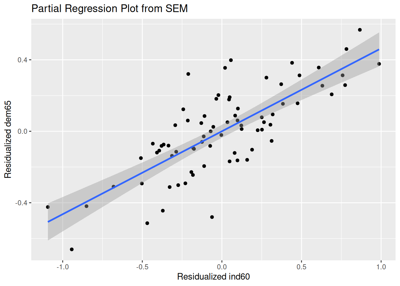
For troubleshooting warnings in SEM, follow the guidance here: https://isaactpetersen.github.io/Principles-Psychological-Assessment/factor-analysis-pca.html#sec-troubleshooting-factorAnalysis.
For various aspects/diagnostics of the model fit object that you can extract, see the lavaan::lavInspect() function.
Here is how to perform various concrete steps:
psych::describe(longitudinalMI)cor(longitudinalMI, use = "pairwise.complete.obs")petersenlab::cor.table(longitudinalMI)hist(longitudinalMI$JOBSAT11)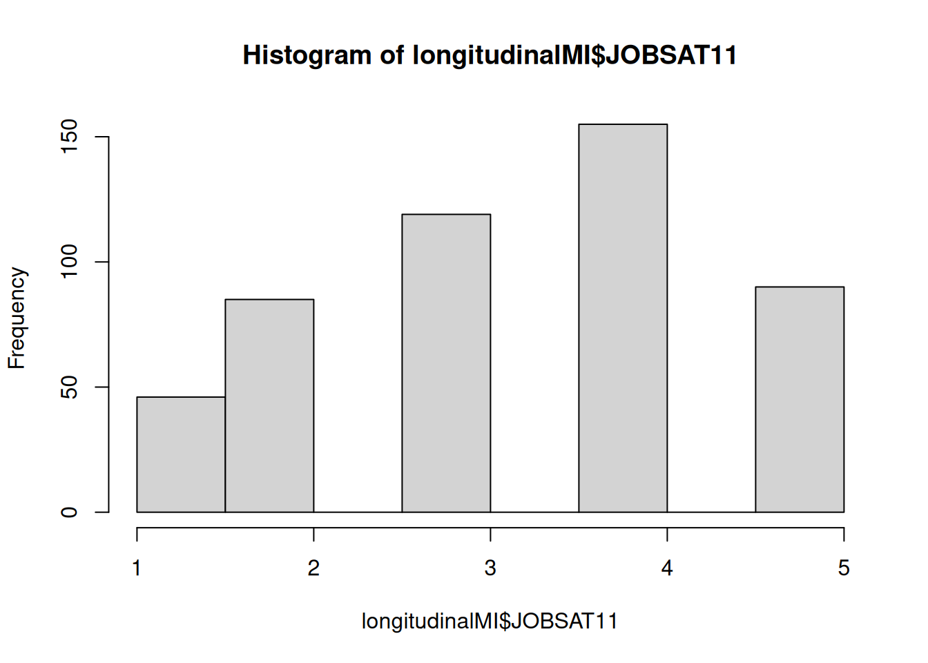
lavInspect(configuralInvariance_fit, "converged")[1] TRUEfitMeasures(configuralInvariance_fit, "df") df
288 parameterEstimates(configuralInvariance_fit, standardized = TRUE)Examine the variance-covariance matrix of the model parameters:
lavInspect(configuralInvariance_fit, "vcov")
cov2cor(lavInspect(configuralInvariance_fit, "vcov"))lavInspect(configuralInvariance_fit, "sigma.hat")
cov2cor(lavInspect(configuralInvariance_fit, "sigma.hat"))lavInspect(configuralInvariance_fit, "cov.lv") jbst_1 jbst_2 jbst_3 redy_1 redy_2 redy_3 cmmt_1 cmmt_2 cmmt_3
jobsat_1 1.000
jobsat_2 0.436 0.933
jobsat_3 0.325 0.381 0.748
ready_1 0.542 0.198 0.201 1.000
ready_2 0.286 0.508 0.272 0.404 1.108
ready_3 0.176 0.193 0.451 0.323 0.515 0.952
commit_1 0.581 0.278 0.182 0.452 0.270 0.175 1.000
commit_2 0.380 0.584 0.265 0.282 0.694 0.298 0.632 1.114
commit_3 0.237 0.260 0.480 0.230 0.309 0.452 0.427 0.583 0.916cov2cor(lavInspect(configuralInvariance_fit, "cov.lv")) jbst_1 jbst_2 jbst_3 redy_1 redy_2 redy_3 cmmt_1 cmmt_2 cmmt_3
jobsat_1 1.000
jobsat_2 0.451 1.000
jobsat_3 0.375 0.456 1.000
ready_1 0.542 0.205 0.232 1.000
ready_2 0.271 0.500 0.298 0.383 1.000
ready_3 0.181 0.205 0.534 0.331 0.501 1.000
commit_1 0.581 0.288 0.210 0.452 0.256 0.180 1.000
commit_2 0.360 0.573 0.290 0.267 0.625 0.289 0.598 1.000
commit_3 0.248 0.281 0.580 0.240 0.307 0.484 0.447 0.577 1.000eigen(lavInspect(configuralInvariance_fit, "vcov"))$valueseigen(lavInspect(configuralInvariance_fit, "sigma.hat"))$values [1] 9.9623877 3.4928485 2.9415770 2.5419423 2.3628163 1.3778102 1.1602808
[8] 1.0025555 0.8310505 0.5870375 0.5555553 0.5453167 0.5425452 0.5380872
[15] 0.5378393 0.5364108 0.5250124 0.5165407 0.5157697 0.5129455 0.5097659
[22] 0.5081709 0.5060723 0.5019531 0.4878037 0.4862790 0.4713891eigen(lavInspect(configuralInvariance_fit, "cov.lv"))$values[1] 3.9816267 1.2139721 0.9865842 0.8751060 0.7548242 0.3548652 0.2564884
[8] 0.2033528 0.1448842modindices(configuralInvariance_fit, sort = TRUE)fitMeasures(configuralInvariance_fit) npar fmin
117.000 0.779
chisq df
770.816 288.000
pvalue chisq.scaled
0.000 783.291
df.scaled pvalue.scaled
288.000 0.000
chisq.scaling.factor baseline.chisq
0.984 6697.063
baseline.df baseline.pvalue
351.000 0.000
baseline.chisq.scaled baseline.df.scaled
6541.933 351.000
baseline.pvalue.scaled baseline.chisq.scaling.factor
0.000 1.024
cfi tli
0.924 0.907
cfi.scaled tli.scaled
0.920 0.902
cfi.robust tli.robust
0.923 0.906
nnfi rfi
0.907 0.860
nfi pnfi
0.885 0.726
ifi rni
0.925 0.924
nnfi.scaled rfi.scaled
0.902 0.854
nfi.scaled pnfi.scaled
0.880 0.722
ifi.scaled rni.scaled
0.921 0.920
nnfi.robust rni.robust
0.906 0.923
logl unrestricted.logl
-17716.771 -17331.363
aic bic
35667.543 36159.476
ntotal bic2
495.000 35788.115
scaling.factor.h1 scaling.factor.h0
0.998 0.935
rmsea rmsea.ci.lower
0.058 0.053
rmsea.ci.upper rmsea.ci.level
0.063 0.900
rmsea.pvalue rmsea.close.h0
0.003 0.050
rmsea.notclose.pvalue rmsea.notclose.h0
0.000 0.080
rmsea.scaled rmsea.ci.lower.scaled
0.059 0.054
rmsea.ci.upper.scaled rmsea.pvalue.scaled
0.064 0.002
rmsea.notclose.pvalue.scaled rmsea.robust
0.000 0.058
rmsea.ci.lower.robust rmsea.ci.upper.robust
0.054 0.063
rmsea.pvalue.robust rmsea.notclose.pvalue.robust
0.002 0.000
rmr rmr_nomean
0.041 0.042
srmr srmr_bentler
0.032 0.032
srmr_bentler_nomean crmr
0.033 0.033
crmr_nomean srmr_mplus
0.034 0.032
srmr_mplus_nomean cn_05
0.033 212.007
cn_01 gfi
223.678 0.967
agfi pgfi
0.954 0.688
mfi ecvi
0.614 2.030
attr(,"scaled.test")
[1] "yuan.bentler.mplus"R version 4.6.1 (2026-06-24)
Platform: x86_64-pc-linux-gnu
Running under: Ubuntu 24.04.4 LTS
Matrix products: default
BLAS: /usr/lib/x86_64-linux-gnu/openblas-pthread/libblas.so.3
LAPACK: /usr/lib/x86_64-linux-gnu/openblas-pthread/libopenblasp-r0.3.26.so; LAPACK version 3.12.0
locale:
[1] LC_CTYPE=C.UTF-8 LC_NUMERIC=C LC_TIME=C.UTF-8
[4] LC_COLLATE=C.UTF-8 LC_MONETARY=C.UTF-8 LC_MESSAGES=C.UTF-8
[7] LC_PAPER=C.UTF-8 LC_NAME=C LC_ADDRESS=C
[10] LC_TELEPHONE=C LC_MEASUREMENT=C.UTF-8 LC_IDENTIFICATION=C
time zone: UTC
tzcode source: system (glibc)
attached base packages:
[1] stats graphics grDevices utils datasets methods base
other attached packages:
[1] ggforce_0.5.0 lubridate_1.9.5 forcats_1.0.1 stringr_1.6.0
[5] dplyr_1.2.1 purrr_1.2.2 readr_2.2.0 tidyr_1.3.2
[9] tibble_3.3.1 ggplot2_4.0.3 tidyverse_2.0.0 MBESS_5.0.1
[13] lcsm_0.3.2 lavaangui_0.4.0 lavaanPlot_0.8.1 semPlot_1.1.8
[17] semTools_0.5-8 lavaan_0.6-21
loaded via a namespace (and not attached):
[1] RColorBrewer_1.1-3 rstudioapi_0.19.0 jsonlite_2.0.0
[4] magrittr_2.0.5 farver_2.1.2 nloptr_2.2.1
[7] rmarkdown_2.31 vctrs_0.7.3 minqa_1.2.8
[10] base64enc_0.1-6 htmltools_0.5.9 Formula_1.2-5
[13] htmlwidgets_1.6.4 plyr_1.8.9 igraph_2.3.3
[16] mime_0.13 lifecycle_1.0.5 pkgconfig_2.0.3
[19] Matrix_1.7-5 R6_2.6.1 fastmap_1.2.0
[22] rbibutils_2.4.1 shiny_1.14.0 digest_0.6.39
[25] OpenMx_2.22.11 fdrtool_1.2.18 colorspace_2.1-2
[28] Hmisc_5.2-6 labeling_0.4.3 timechange_0.4.0
[31] polyclip_1.10-7 abind_1.4-8 mgcv_1.9-4
[34] compiler_4.6.1 withr_3.0.3 glasso_1.11
[37] htmlTable_2.5.0 S7_0.2.2 backports_1.5.1
[40] carData_3.0-6 DBI_1.3.0 psych_2.6.5
[43] MASS_7.3-65 corpcor_1.6.10 gtools_3.9.5
[46] petersenlab_1.2.3 tools_4.6.1 pbivnorm_0.6.0
[49] foreign_0.8-91 otel_0.2.0 zip_3.0.0
[52] httpuv_1.6.17 nnet_7.3-20 glue_1.8.1
[55] quadprog_1.5-8 DiagrammeR_1.0.12 nlme_3.1-169
[58] promises_1.5.0 lisrelToR_0.3 grid_4.6.1
[61] checkmate_2.3.4 cluster_2.1.8.2 reshape2_1.4.5
[64] generics_0.1.4 gtable_0.3.6 tzdb_0.5.0
[67] data.table_1.18.4 hms_1.1.4 sem_3.1-16
[70] pillar_1.11.1 rockchalk_1.8.164 later_1.4.8
[73] mitools_2.4 splines_4.6.1 tweenr_2.0.3
[76] lattice_0.22-9 kutils_1.73 tidyselect_1.2.1
[79] pbapply_1.7-4 mix_1.0-13 knitr_1.51
[82] reformulas_0.4.4 gridExtra_2.3.1 stats4_4.6.1
[85] xfun_0.60 qgraph_1.9.8 arm_1.15-3
[88] visNetwork_2.1.4 stringi_1.8.7 yaml_2.3.12
[91] boot_1.3-32 evaluate_1.0.5 mi_1.2
[94] cli_3.6.6 RcppParallel_5.1.11-2 rpart_4.1.27
[97] xtable_1.8-8 Rdpack_2.6.6 Rcpp_1.1.2
[100] coda_0.19-4.1 png_0.1-9 XML_3.99-0.23
[103] parallel_4.6.1 jpeg_0.1-11 lme4_2.0-1
[106] viridisLite_0.4.3 mvtnorm_1.4-1 scales_1.4.0
[109] openxlsx_4.2.8.1 rlang_1.3.0 mnormt_2.1.2