Exploratory Data Analysis

1 Rationale

Exploratory data analysis is important for understanding your data, checking for data issues/errors, and checking assumptions for different statistical models.

LOOK AT YOUR DATA—this is one of the most overlooked steps in data analysis!

2 Preamble

2.1 Install Libraries

Code

#install.packages("remotes")
#remotes::install_github("DevPsyLab/petersenlab")

2.2 Load Libraries

Code

library("petersenlab")
library("car")
library("vioplot")
library("ellipse")
library("nlme")
library("effects")
library("corrplot")
library("ggplot2")
library("psych")
library("tidyverse")
library("purrr")
library("naniar")
library("mvnormtest")
library("ggExtra")
library("XICOR")

3 Simulate Data

Code

set.seed(52242)

n <- 1000

ID <- rep(1:100, each = 10)
predictor <- rbeta(n, 1.5, 5) * 100
outcome <- predictor + rnorm(n, mean = 0, sd = 20) + 50

predictorOverplot <- sample(1:50, n, replace = TRUE)
outcomeOverplot <- predictorOverplot + sample(1:75, n, replace = TRUE)

categorical1 <- sample(1:5, size = n, replace = TRUE)
categorical2 <- sample(1:5, size = n, replace = TRUE)

mydata <- data.frame(
  ID = ID,
  predictor = predictor,
  outcome = outcome,
  predictorOverplot = predictorOverplot,
  outcomeOverplot = outcomeOverplot,
  categorical1 = categorical1,
  categorical2 = categorical2)

mydata[sample(1:n, size = 10), "predictor"] <- NA
mydata[sample(1:n, size = 10), "outcome"] <- NA
mydata[sample(1:n, size = 10), "predictorOverplot"] <- NA
mydata[sample(1:n, size = 10), "outcomeOverplot"] <- NA
mydata[sample(1:n, size = 30), "categorical1"] <- NA
mydata[sample(1:n, size = 70), "categorical2"] <- NA

4 Descriptive statistics

Code

round(data.frame(psych::describe(mydata)), 2)

4.1 Sample

Check the sample size (N)
- Is the sample size in the data the expected sample size? Are there cases (participants) that are missing? Are there cases that should not be there?
- Here is the sample size:

Code

length(unique(mydata$ID))

[1] 100

Check the extent of missingness
- How much data are missing in the model variables—including the predictor, outcome, and covariates?
- Here are the proportion of missing data in each variable:

Code

map(mydata, ~mean(is.na(.))) |> t |> t

Error in t: The pipe operator requires a function call as RHS (<input>:1:33)

4.2 Distribution

Frequencies
- Examine the frequencies of categorical variables:

Code

mydata |> 
  select(categorical1, categorical2) |>
  sapply(function(x) table(x, useNA = "always")) |> 
  t()

               1   2   3   4   5 <NA>
categorical1 196 204 191 199 180   30
categorical2 195 179 193 202 161   70

4.3 Central Tendency

Mean

Code

round(colMeans(mydata, na.rm = TRUE), 2)

               ID         predictor           outcome predictorOverplot 
            50.50             22.64             73.36             25.54 
  outcomeOverplot      categorical1      categorical2 
            63.53              2.96              2.95

Code

round(apply(mydata, 2, function(x) mean(x, na.rm = TRUE)), 2)

               ID         predictor           outcome predictorOverplot 
            50.50             22.64             73.36             25.54 
  outcomeOverplot      categorical1      categorical2 
            63.53              2.96              2.95

Code

mydata |> 
  summarise(across(everything(),
                   .fns = list(mean = ~ mean(., na.rm = TRUE)))) |> 
  round(., 2)

Error:
! object '.' not found

Median

Code

round(apply(mydata, 2, function(x) median(x, na.rm = TRUE)), 2)

               ID         predictor           outcome predictorOverplot 
            50.50             19.61             73.17             26.00 
  outcomeOverplot      categorical1      categorical2 
            63.00              3.00              3.00

Code

mydata |> 
  summarise(across(everything(),
                   .fns = list(median = ~ median(., na.rm = TRUE)))) |> 
  round(., 2)

Error:
! object '.' not found

Mode

Code

round(apply(mydata, 2, function(x) Mode(x, multipleModes = "mean")), 2)

               ID         predictor           outcome predictorOverplot 
            50.50             22.64             73.36             35.00 
  outcomeOverplot      categorical1      categorical2 
            63.33              2.00              4.00

Code

mydata |> 
  summarise(across(everything(),
                   .fns = list(mode = ~ Mode(., multipleModes = "mean")))) |> 
  round(., 2)

Error:
! object '.' not found

Compute all of these measures of central tendency:

Code

mydata |> 
  summarise(across(everything(),
                   .fns = list(mean = ~ mean(., na.rm = TRUE),
                               median = ~ median(., na.rm = TRUE),
                               mode = ~ Mode(., multipleModes = "mean")),
                   .names = "{.col}.{.fn}")) |> 
  round(., 2) |> 
  pivot_longer(cols = everything(),
               names_to = c("variable","index"),
               names_sep = "\\.") |> 
  pivot_wider(names_from = index,
              values_from = value)

Error:
! object '.' not found

4.4 Dispersion

Standard deviation
Observed minimum and maximum (vis-à-vis possible minimum and maximum)
Skewness
Kurtosis

Compute all of these measures of dispersion:

Code

mydata |> 
  summarise(across(everything(),
                   .fns = list(SD = ~ sd(., na.rm = TRUE),
                               min = ~ min(., na.rm = TRUE),
                               max = ~ max(., na.rm = TRUE),
                               skewness = ~ skew(., na.rm = TRUE),
                               kurtosis = ~ kurtosi(., na.rm = TRUE)),
                   .names = "{.col}.{.fn}")) |> 
  round(., 2) |> 
  pivot_longer(cols = everything(),
               names_to = c("variable","index"),
               names_sep = "\\.") |> 
  pivot_wider(names_from = index,
              values_from = value)

Error:
! object '.' not found

Consider transforming data if skewness > |0.8| or if kurtosis > |3.0|.

4.5 Summary Statistics

Add summary statistics to the bottom of correlation matrices in papers:

Code

cor.table(mydata, type = "manuscript")

Code

summaryTable <- mydata |> 
  summarise(across(everything(),
                   .fns = list(n = ~ length(na.omit(.)),
                               missingness = ~ mean(is.na(.)) * 100,
                               M = ~ mean(., na.rm = TRUE),
                               SD = ~ sd(., na.rm = TRUE),
                               min = ~ min(., na.rm = TRUE),
                               max = ~ max(., na.rm = TRUE),
                               skewness = ~ skew(., na.rm = TRUE),
                               kurtosis = ~ kurtosi(., na.rm = TRUE)),
                   .names = "{.col}.{.fn}")) |>  
  pivot_longer(cols = everything(),
               names_to = c("variable","index"),
               names_sep = "\\.") |> 
  pivot_wider(names_from = index,
              values_from = value)

summaryTableTransposed <- summaryTable[-1] |> 
  t() |> 
  as.data.frame() |> 
  setNames(summaryTable$variable) |> 
  round(., digits = 2)

Error:
! object '.' not found

Code

summaryTableTransposed

Error:
! object 'summaryTableTransposed' not found

4.6 Distribution Plots

See here for resources for creating figures in R.

4.6.1 Histogram

4.6.1.1 Base R

Code

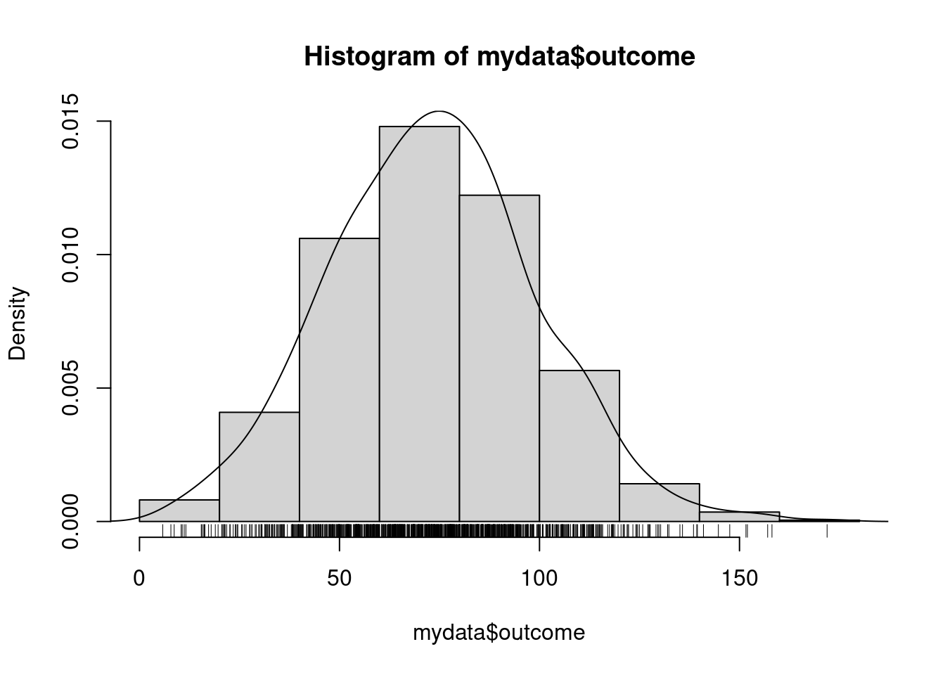
hist(mydata$outcome)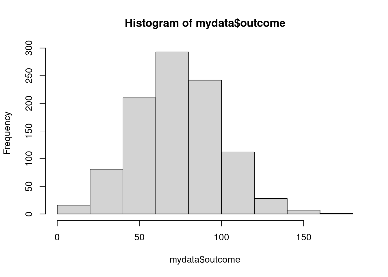

4.6.1.2 `ggplot2`

Code

ggplot(mydata, aes(x = outcome)) +
  geom_histogram(color = 1)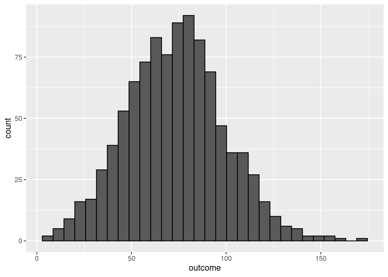

4.6.2 Histogram overlaid with density plot and rug plot

4.6.2.1 Base R

Code

hist(mydata$outcome, prob = TRUE)
lines(density(mydata$outcome, na.rm = TRUE))
rug(mydata$outcome)

4.6.2.2 `ggplot2`

Code

ggplot(mydata, aes(x = outcome)) +
  geom_histogram(aes(y = after_stat(density)), color = 1) +
  geom_density() +
  geom_rug()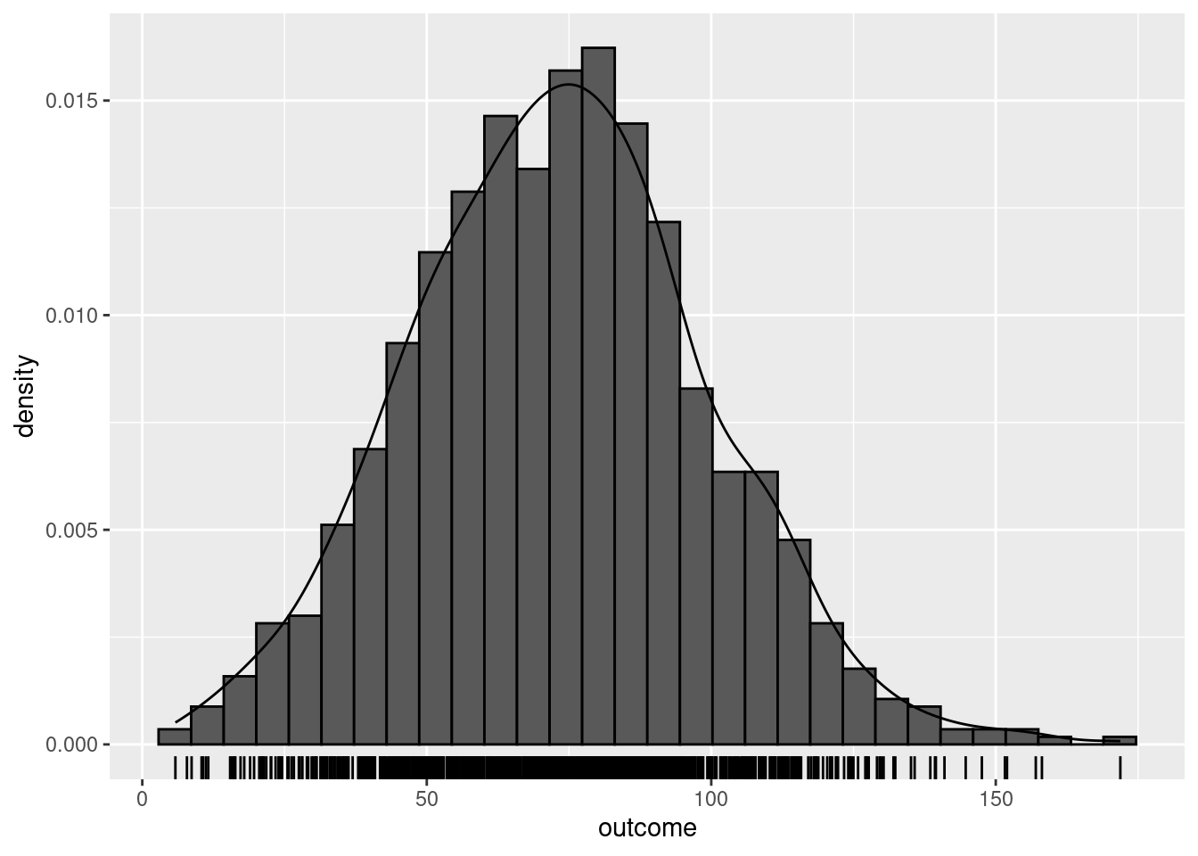

4.6.3 Density Plot

4.6.3.1 Base R

Code

plot(density(mydata$outcome, na.rm = TRUE))

4.6.3.2 `ggplot2`

Code

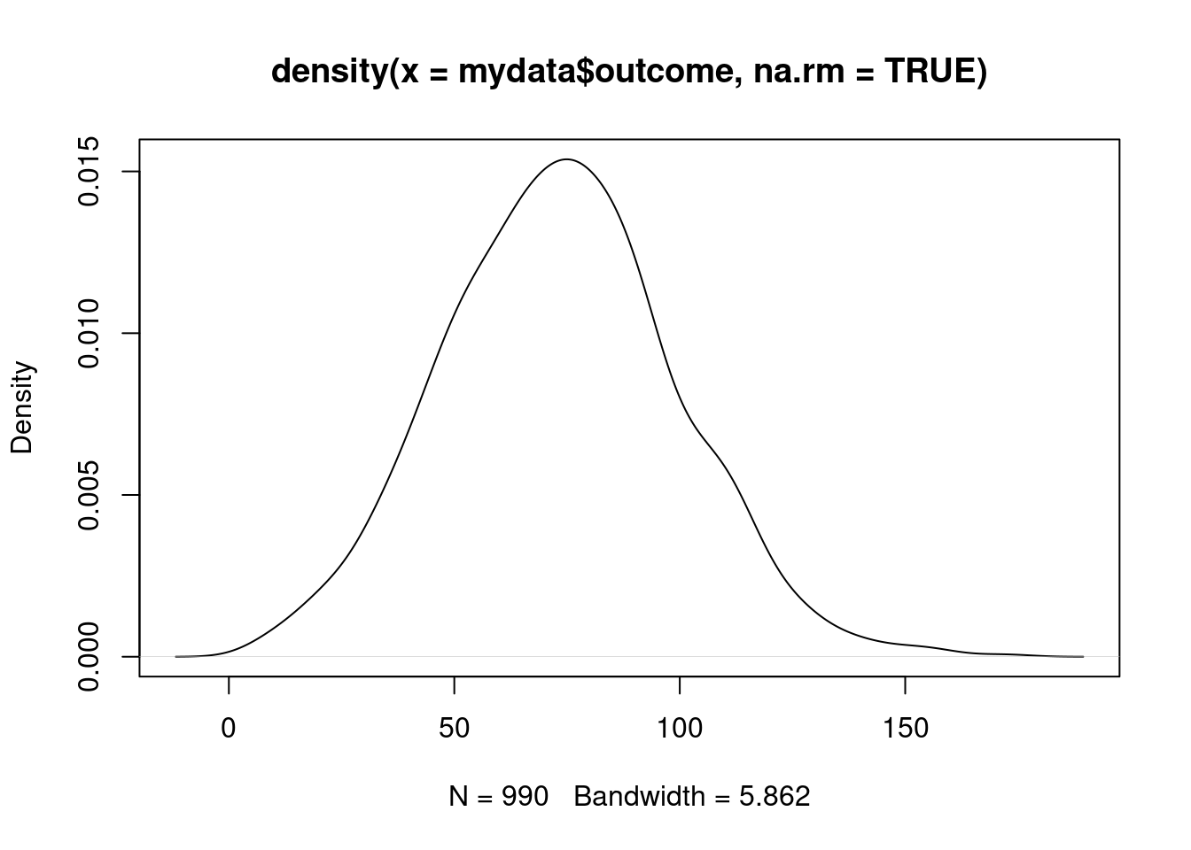
ggplot(mydata, aes(x = outcome)) +
  geom_density()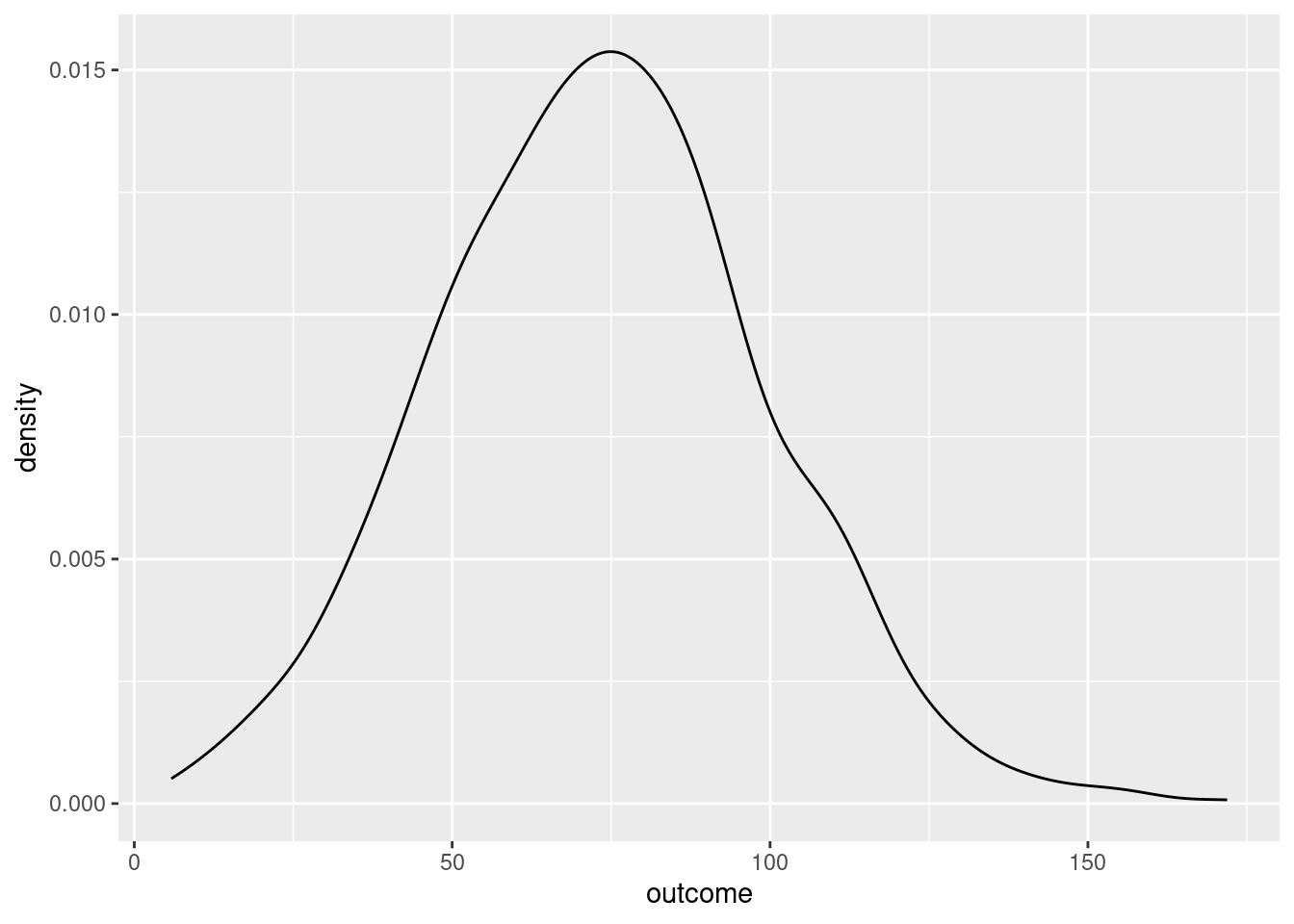

4.6.4 Box and whisker plot (boxplot)

4.6.4.1 Base R

Code

boxplot(mydata$outcome, horizontal = TRUE)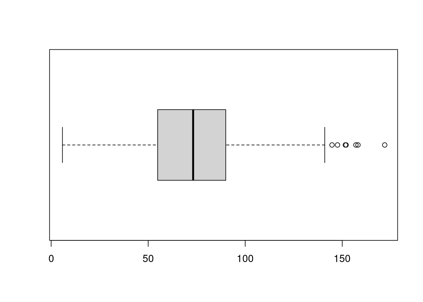

4.6.4.2 `ggplot2`

Code

ggplot(mydata, aes(x = outcome)) +
  geom_boxplot()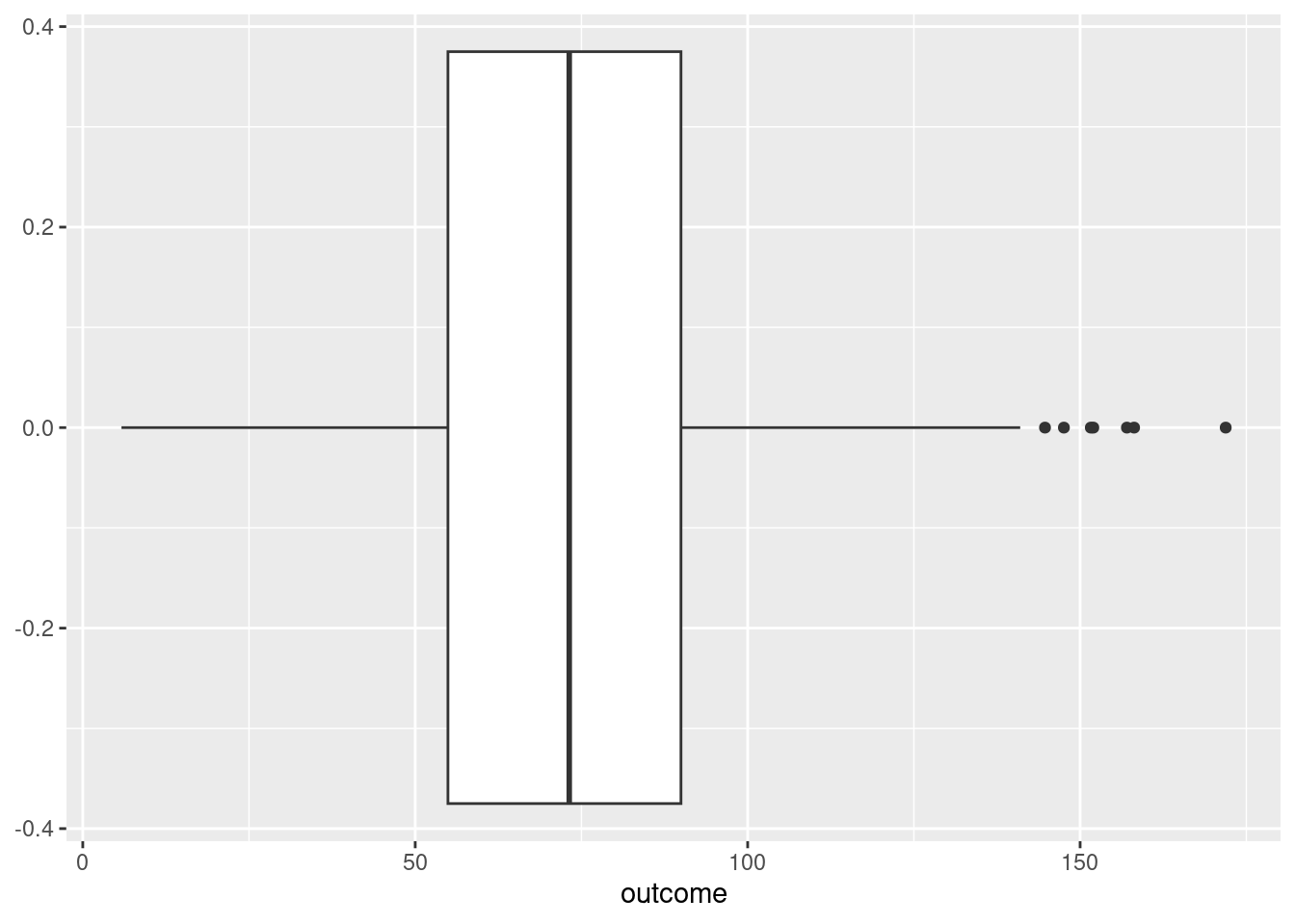

4.6.5 Violin plot

4.6.5.1 Base R

Code

vioplot(na.omit(mydata$outcome), horizontal = TRUE)

4.6.5.2 `ggplot2`

Code

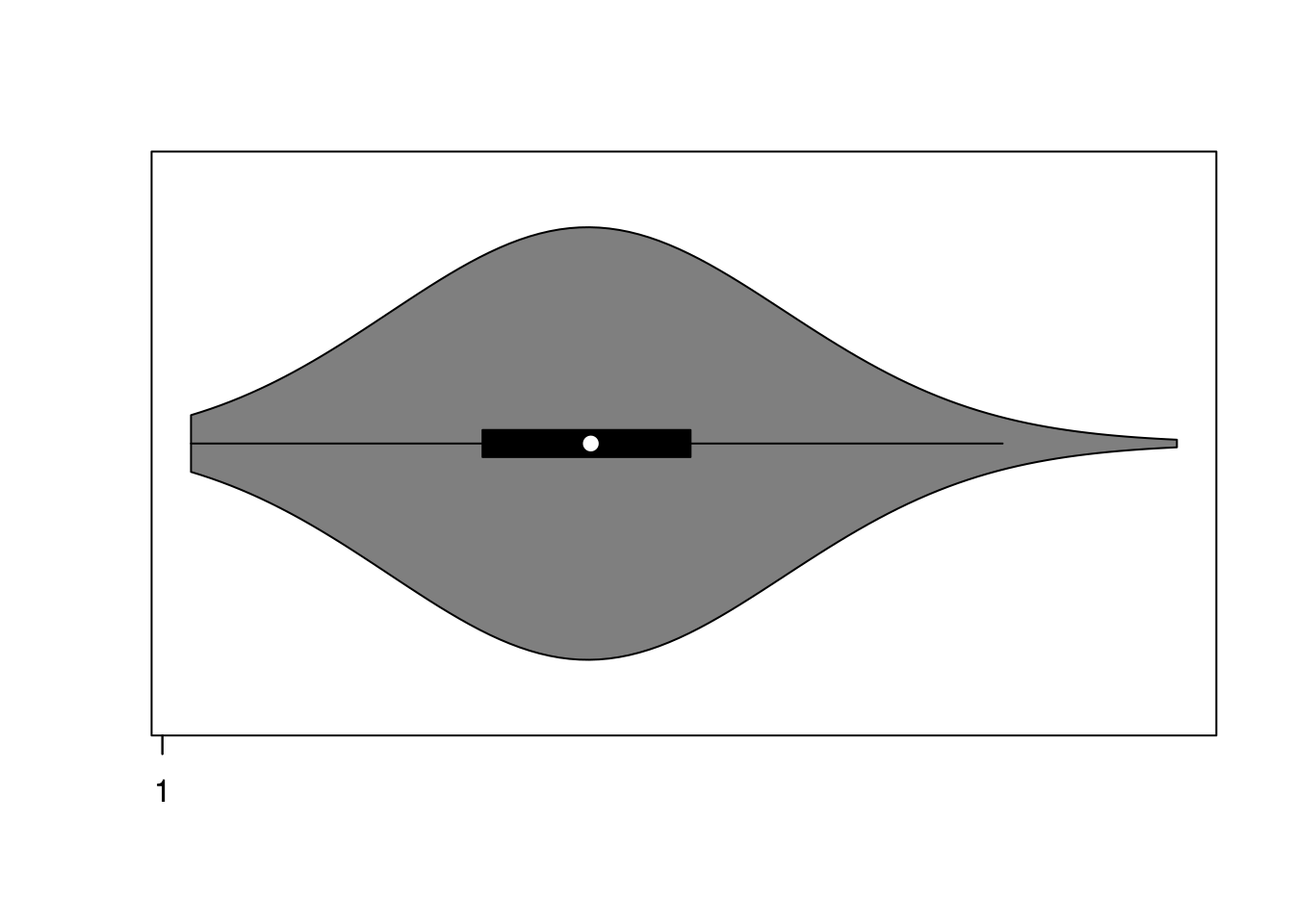
ggplot(mydata, aes(x = "", y = outcome)) +
  geom_violin()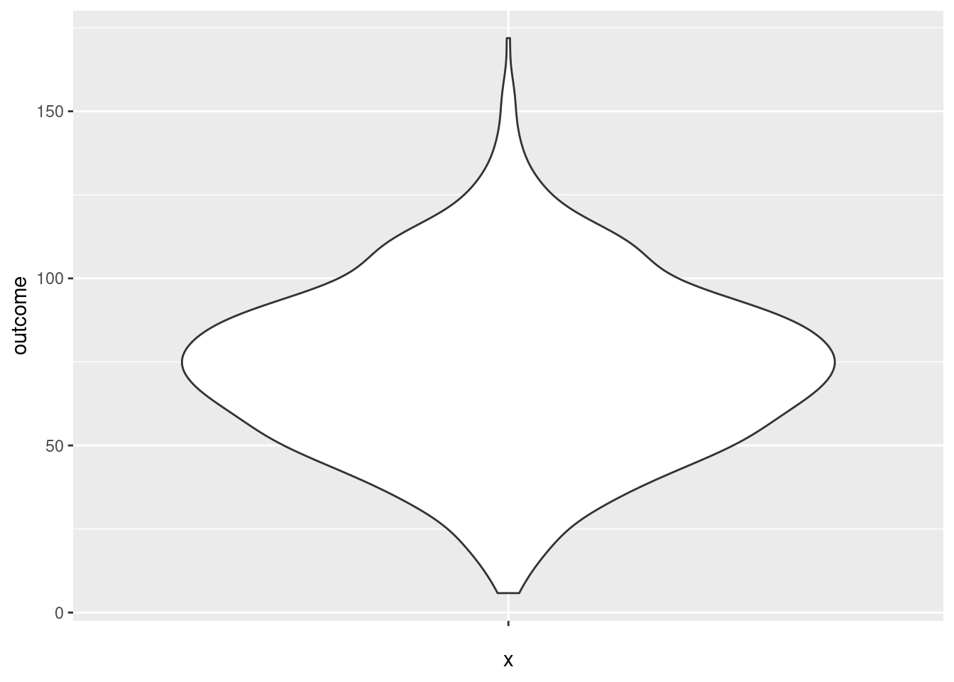

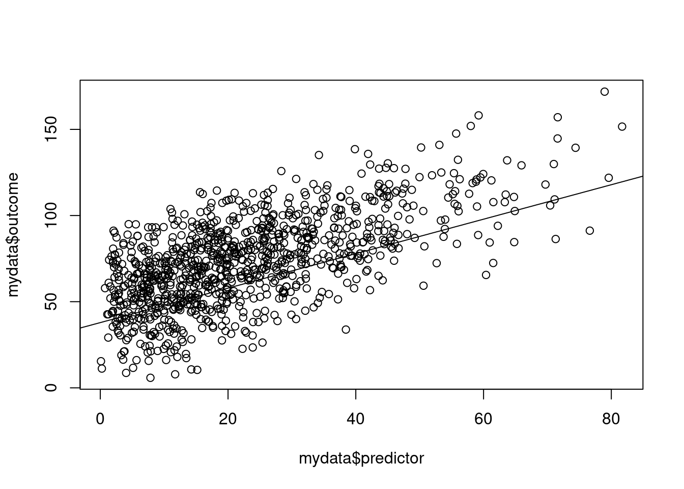
5 Bivariate Associations

For more advanced scatterplots, see here. For an overview of correlation analysis, see here.

5.1 Correlation Coefficients

5.1.1 Pearson Correlation

Code

cor(mydata, use = "pairwise.complete.obs")

                            ID    predictor     outcome predictorOverplot
ID                 1.000000000 -0.019094589 -0.02501796        0.02984671
predictor         -0.019094589  1.000000000  0.63517610        0.04350431
outcome           -0.025017962  0.635176098  1.00000000        0.02976820
predictorOverplot  0.029846711  0.043504314  0.02976820        1.00000000
outcomeOverplot    0.003150872  0.043344473  0.06289224        0.56564445
categorical1       0.040442534 -0.002422711 -0.01532232        0.02498938
categorical2       0.008920415 -0.046927177 -0.01868628        0.03880135
                  outcomeOverplot categorical1 categorical2
ID                    0.003150872  0.040442534  0.008920415
predictor             0.043344473 -0.002422711 -0.046927177
outcome               0.062892238 -0.015322318 -0.018686282
predictorOverplot     0.565644447  0.024989385  0.038801346
outcomeOverplot       1.000000000  0.011871644  0.043682632
categorical1          0.011871644  1.000000000 -0.086310192
categorical2          0.043682632 -0.086310192  1.000000000

Code

cor.test( ~ predictor + outcome, data = mydata)


    Pearson's product-moment correlation

data:  predictor and outcome
t = 25.718, df = 978, p-value < 2.2e-16
alternative hypothesis: true correlation is not equal to 0
95 percent confidence interval:
 0.5962709 0.6711047
sample estimates:
      cor 
0.6351761

Code

cor.table(mydata)

5.1.2 Spearman Correlation

Code

cor(mydata, use = "pairwise.complete.obs", method = "spearman")

                            ID   predictor     outcome predictorOverplot
ID                 1.000000000 -0.01181085 -0.02805450        0.02925155
predictor         -0.011810853  1.00000000  0.60003760        0.02672008
outcome           -0.028054497  0.60003760  1.00000000        0.02460831
predictorOverplot  0.029251546  0.02672008  0.02460831        1.00000000
outcomeOverplot    0.001416626  0.03278463  0.07073642        0.54841297
categorical1       0.040888369 -0.01162260 -0.01906631        0.02350886
categorical2       0.009137467 -0.03763251 -0.02273699        0.04062487
                  outcomeOverplot categorical1 categorical2
ID                    0.001416626   0.04088837  0.009137467
predictor             0.032784628  -0.01162260 -0.037632515
outcome               0.070736421  -0.01906631 -0.022736992
predictorOverplot     0.548412967   0.02350886  0.040624873
outcomeOverplot       1.000000000   0.01505255  0.044184959
categorical1          0.015052553   1.00000000 -0.086290083
categorical2          0.044184959  -0.08629008  1.000000000

Code

cor.test( ~ predictor + outcome, data = mydata, method = "spearman")


    Spearman's rank correlation rho

data:  predictor and outcome
S = 62740170, p-value < 2.2e-16
alternative hypothesis: true rho is not equal to 0
sample estimates:
      rho 
0.6000376

Code

cor.table(mydata, correlation = "spearman")

5.1.3 Xi (\(\xi\))

Xi (\(\xi\)) is an index of the degree of dependence between two variables, which is useful as an index of nonlinear correlation.

Chatterjee, S. (2021). A new coefficient of correlation. Journal of the American Statistical Association, 116(536), 2009-2022. https://doi.org/10.1080/01621459.2020.1758115

Code

calculateXI(
  mydata$predictor,
  mydata$outcome)

[1] 0.2319062

5.2 Scatterplot

5.2.1 Base R

Code

plot(
  mydata$predictor,
  mydata$outcome)
abline(lm(
  outcomeOverplot ~ predictorOverplot,
  data = mydata,
  na.action = "na.exclude"))

5.2.2 `ggplot2`

Code

ggplot(mydata, aes(x = predictor, y = outcome)) + 
  geom_point() +
  geom_smooth(method = "lm", se = TRUE)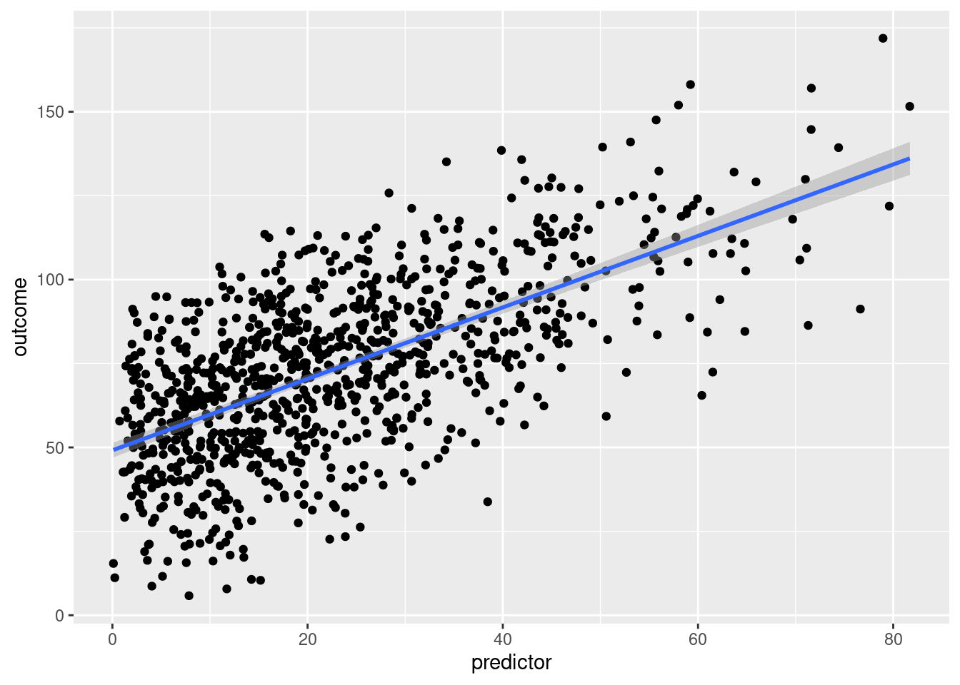

5.3 Scatterplot with Marginal Density Plot

Code

scatterplot <- 
  ggplot(mydata, aes(x = predictor, y = outcome)) + 
  geom_point() +
  geom_smooth(method = "lm", se = TRUE)

Code

densityMarginal <- ggMarginal(
  scatterplot,
  type = "density",
  xparams = list(fill = "gray"),
  yparams = list(fill = "gray"))

Code

print(densityMarginal, newpage = TRUE)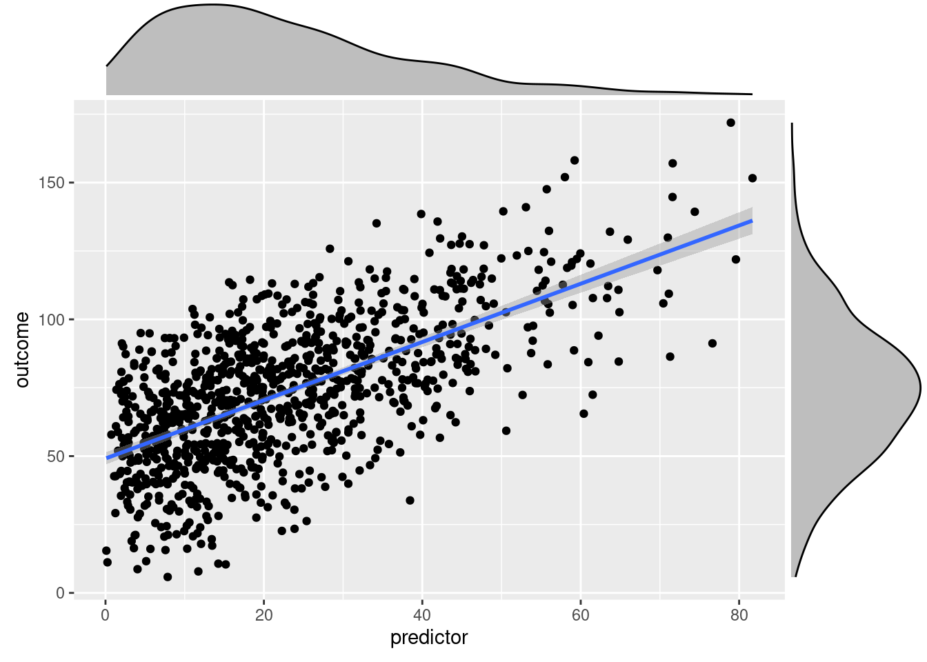

5.4 High Density Scatterplot

Code

ggplot(mydata, aes(x = predictorOverplot, y = outcomeOverplot)) + 
  geom_point(position = "jitter", alpha = 0.3) + 
  geom_density2d()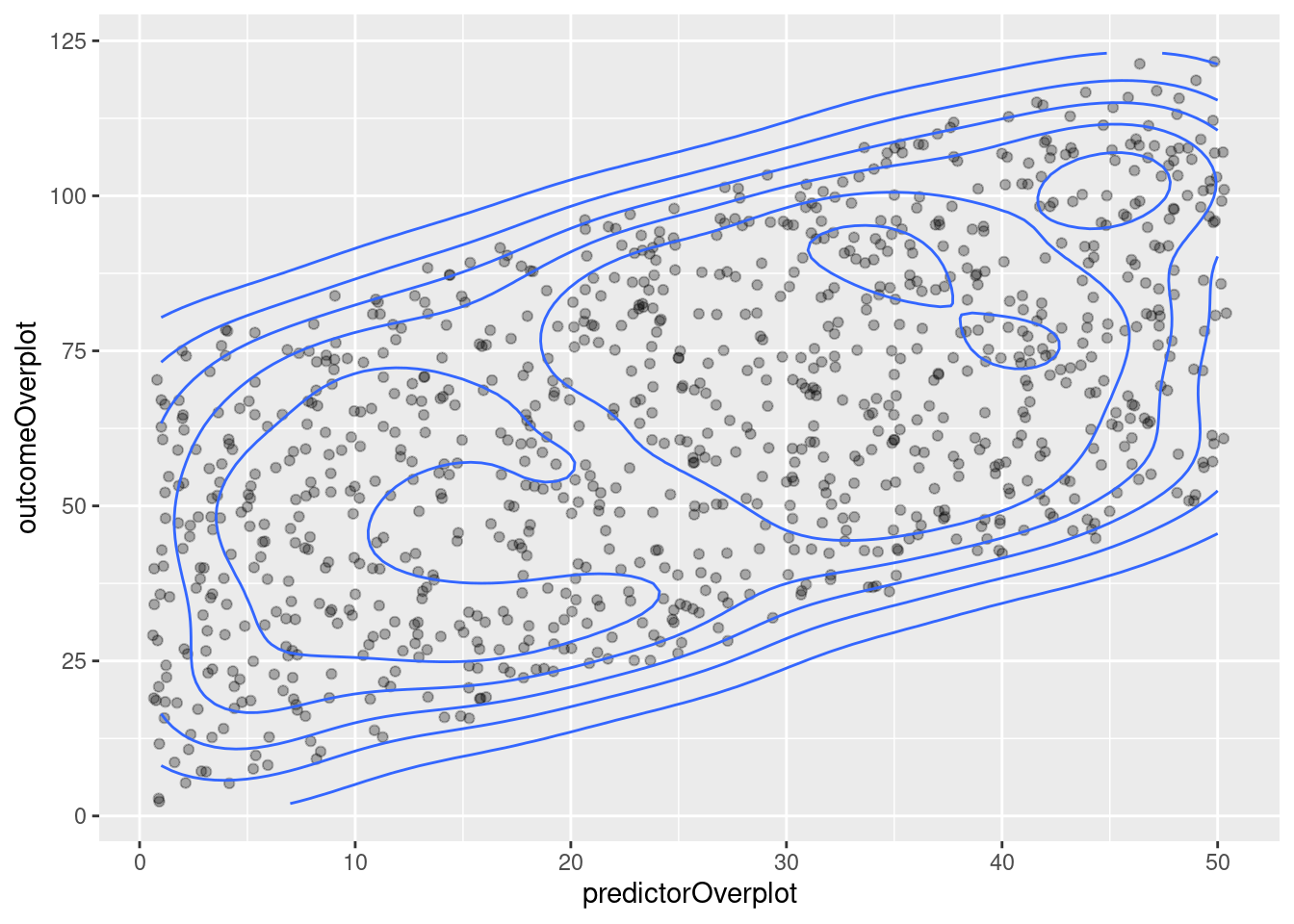

Code

smoothScatter(mydata$predictorOverplot, mydata$outcomeOverplot)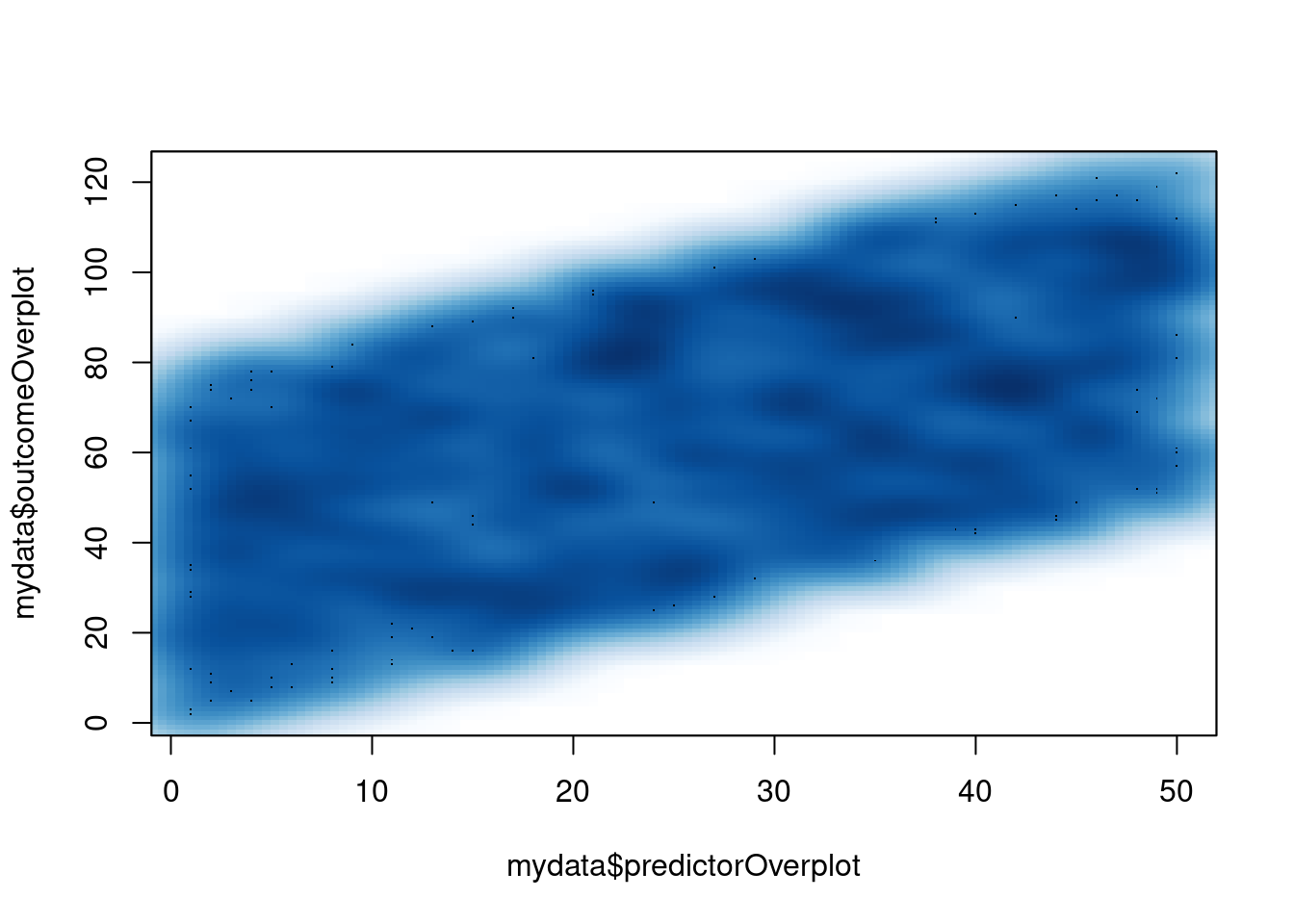

5.5 Data Ellipse

Code

mydata_nomissing <- na.omit(mydata[,c("predictor","outcome")])
dataEllipse(mydata_nomissing$predictor, mydata_nomissing$outcome, levels = c(0.5, .95))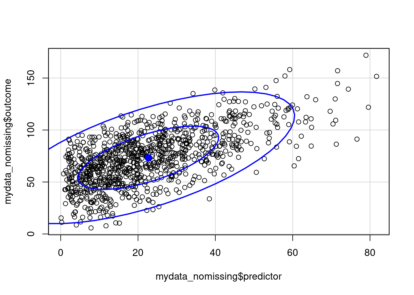

5.6 Visually Weighted Regression

Code

vwReg(outcome ~ predictor, data = mydata)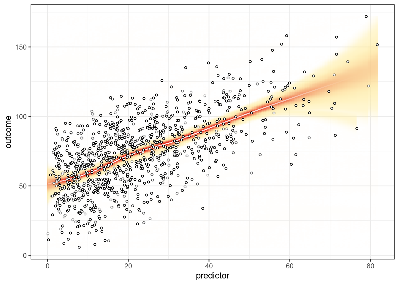

6 Basic inferential statistics

6.1 Tests of Normality

6.1.1 Shapiro-Wilk test of normality

The Shapiro-Wilk test of normality does not accept more than 5000 cases because it will reject the hypothesis that data come from a normal distribution with even slight deviations from normality.

Code

shapiro.test(na.omit(mydata$outcome)) #subset to keep only the first 5000 rows: mydata$outcome[1:5000]


    Shapiro-Wilk normality test

data:  na.omit(mydata$outcome)
W = 0.9971, p-value = 0.06998

6.1.2 Test of multivariate normality

Code

mydata |> 
  na.omit |> 
  t |> 
  mshapiro.test

Error in na.omit: The pipe operator requires a function call as RHS (<input>:2:3)

6.2 Tests of systematic missingness (i.e., whether missingness on a variable depends on other variables)

Generally test:
- Whether data are consistent with a missing completely at random (MCAR) pattern—Little’s MCAR Test
- Whether outcome variable(s) differ as a function of any model variables (predictors and covariates) and as a function of any key demographic characteristics (e.g., sex, ethnicity, socioeconomic status)
- Whether focal predictor variable(s) differ as a function of any model variables (including outcome variable) and as a function of any key demographic characteristics
For instance:
- Whether males are more likely than girls to be missing scores on the dependent variable
- Whether longitudinal attrition is greater in lower socioeconomic status families
If missingness differs systematically as a function of other variables, you can include that variable as a control variable in models, and/or can include that variable in multiple imputation to inform imputed scores for missing values

6.2.1 Little’s MCAR Test

Code

mcar_test(mydata)

6.3 Multivariate Associations

6.3.1 Correlation Matrix

6.3.1.1 Pearson Correlations

Code

cor.table(mydata[,c("predictor","outcome","predictorOverplot","outcomeOverplot")])

Code

cor.table(mydata[,c("predictor","outcome","predictorOverplot","outcomeOverplot")], type = "manuscript")

Code

cor.table(mydata[,c("predictor","outcome","predictorOverplot","outcomeOverplot")], type = "manuscriptBig")

6.3.1.2 Spearman Correlations

Code

cor.table(mydata[,c("predictor","outcome","predictorOverplot","outcomeOverplot")], correlation = "spearman")

Code

cor.table(mydata[,c("predictor","outcome","predictorOverplot","outcomeOverplot")], type = "manuscript", correlation = "spearman")

Code

cor.table(mydata[,c("predictor","outcome","predictorOverplot","outcomeOverplot")], type = "manuscriptBig", correlation = "spearman")

6.3.1.3 Partial Correlations

Examine the associations among variables controlling for a covariate (outcomeOverplot).

Code

partialcor.table(mydata[,c("predictor","outcome","predictorOverplot")], z = mydata[,c("outcomeOverplot")])

Code

partialcor.table(mydata[,c("predictor","outcome","predictorOverplot")], z = mydata[,c("outcomeOverplot")], type = "manuscript")

Code

partialcor.table(mydata[,c("predictor","outcome","predictorOverplot")], z = mydata[,c("outcomeOverplot")], type = "manuscriptBig")

6.3.2 Correlogram

Code

corrplot(cor(mydata[,c("predictor","outcome","predictorOverplot","outcomeOverplot")], use = "pairwise.complete.obs"))

6.3.3 Scatterplot matrix

Code

scatterplotMatrix(~ predictor + outcome + predictorOverplot + outcomeOverplot, data = mydata, use = "pairwise.complete.obs")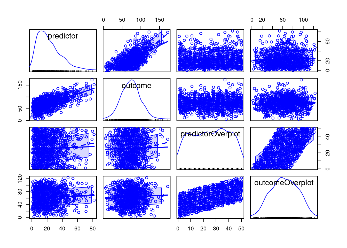

6.3.4 Pairs panels

Code

pairs.panels(mydata[,c("predictor","outcome","predictorOverplot","outcomeOverplot")])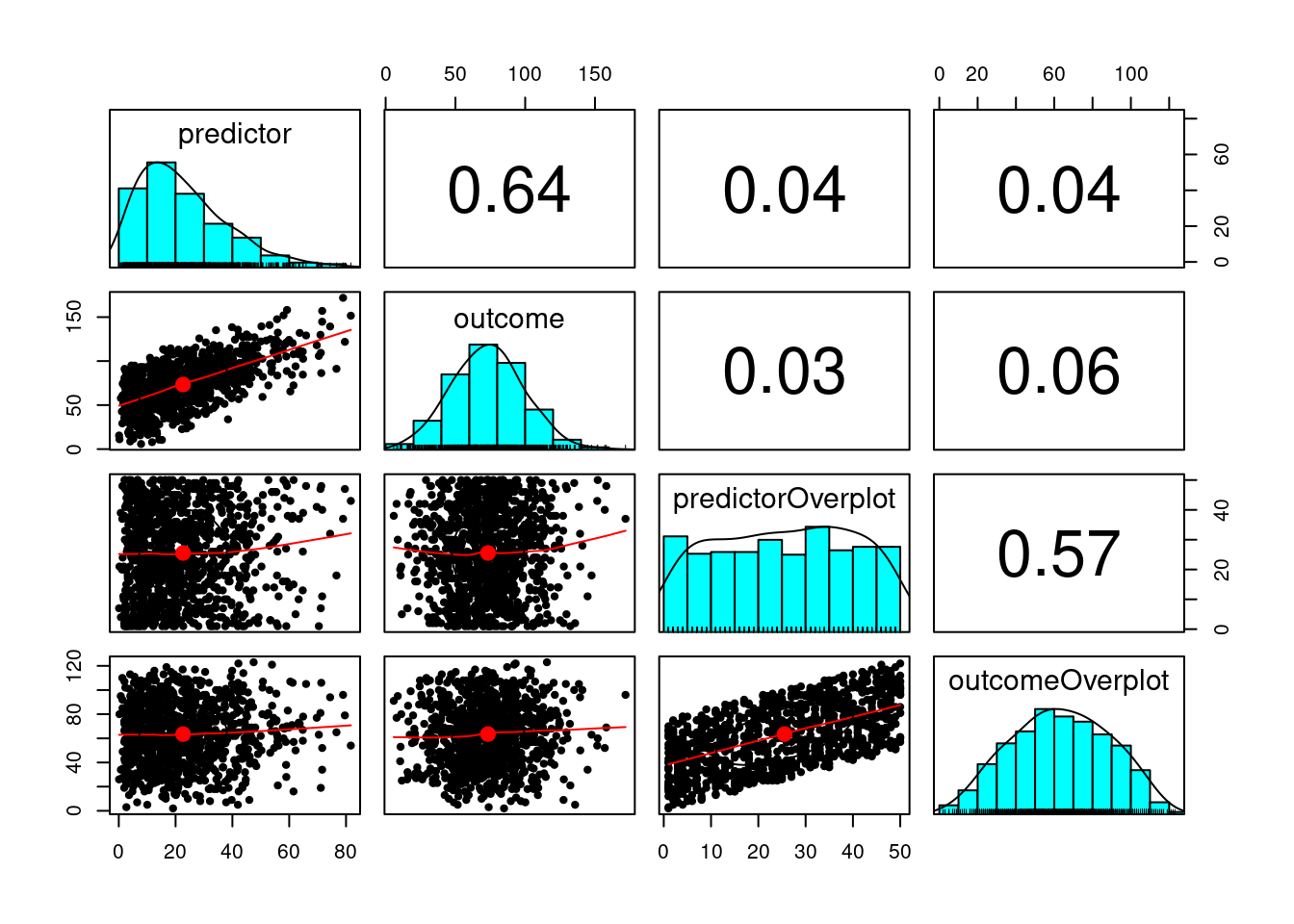

6.4 Effect Plots

6.4.1 Multiple Regression Model

Code

multipleRegressionModel <- lm(outcome ~ predictor + predictorOverplot,
                              data = mydata,
                              na.action = "na.exclude")

allEffects(multipleRegressionModel)

 model: outcome ~ predictor + predictorOverplot

 predictor effect
predictor
      0.1        20        40        60        80 
 49.23335  70.37778  91.62847 112.87915 134.12983 

 predictorOverplot effect
predictorOverplot
       1       10       30       40       50 
73.13937 73.15070 73.17586 73.18845 73.20103

Code

plot(allEffects(multipleRegressionModel))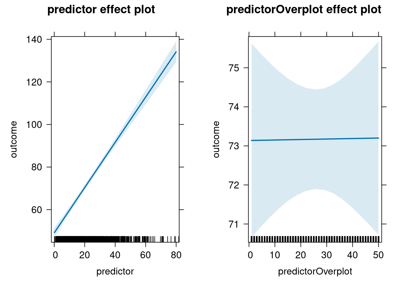

6.4.2 Multilevel Regression Model

Code

multilevelRegressionModel <- lme(outcome ~ predictor + predictorOverplot, random = ~ 1|ID,
                                 method = "ML",
                                 data = mydata,
                                 na.action = "na.exclude")

allEffects(multilevelRegressionModel)

 model: outcome ~ predictor + predictorOverplot

 predictor effect
predictor
      0.1        20        40        60        80 
 49.23335  70.37778  91.62847 112.87915 134.12983 

 predictorOverplot effect
predictorOverplot
       1       10       30       40       50 
73.13937 73.15070 73.17586 73.18845 73.20103

Code

plot(allEffects(multilevelRegressionModel))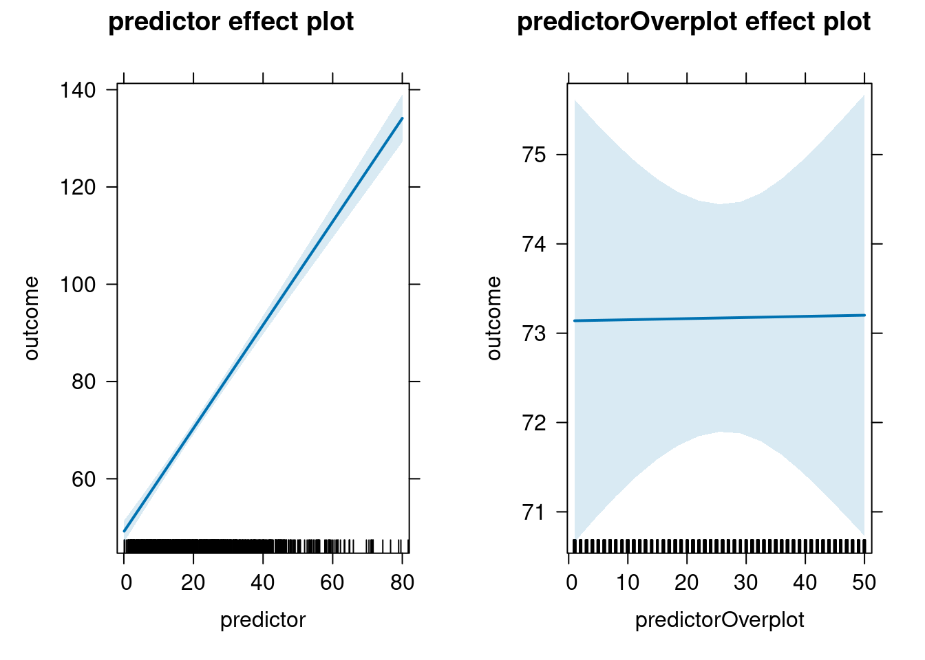

7 Session Info

Code

sessionInfo()

R version 4.6.1 (2026-06-24)
Platform: x86_64-pc-linux-gnu
Running under: Ubuntu 24.04.4 LTS

Matrix products: default
BLAS:   /usr/lib/x86_64-linux-gnu/openblas-pthread/libblas.so.3 
LAPACK: /usr/lib/x86_64-linux-gnu/openblas-pthread/libopenblasp-r0.3.26.so;  LAPACK version 3.12.0

locale:
 [1] LC_CTYPE=C.UTF-8       LC_NUMERIC=C           LC_TIME=C.UTF-8       
 [4] LC_COLLATE=C.UTF-8     LC_MONETARY=C.UTF-8    LC_MESSAGES=C.UTF-8   
 [7] LC_PAPER=C.UTF-8       LC_NAME=C              LC_ADDRESS=C          
[10] LC_TELEPHONE=C         LC_MEASUREMENT=C.UTF-8 LC_IDENTIFICATION=C   

time zone: UTC
tzcode source: system (glibc)

attached base packages:
[1] stats     graphics  grDevices utils     datasets  methods   base     

other attached packages:
 [1] XICOR_0.4.1        ggExtra_0.11.0     mvnormtest_0.1-9-3 naniar_1.1.0      
 [5] lubridate_1.9.5    forcats_1.0.1      stringr_1.6.0      dplyr_1.2.1       
 [9] purrr_1.2.2        readr_2.2.0        tidyr_1.3.2        tibble_3.3.1      
[13] tidyverse_2.0.0    psych_2.6.5        ggplot2_4.0.3      corrplot_0.95     
[17] effects_4.2-5      nlme_3.1-169       ellipse_0.5.0      vioplot_0.5.1     
[21] zoo_1.8-15         sm_2.2-6.0         car_3.1-5          carData_3.0-6     
[25] petersenlab_1.2.3 

loaded via a namespace (and not attached):
 [1] Rdpack_2.6.6       DBI_1.3.0          mnormt_2.1.2       gridExtra_2.3.1   
 [5] rlang_1.3.0        magrittr_2.0.5     otel_0.2.0         compiler_4.6.1    
 [9] mgcv_1.9-4         vctrs_0.7.3        reshape2_1.4.5     quadprog_1.5-8    
[13] pkgconfig_2.0.3    fastmap_1.2.0      backports_1.5.1    labeling_0.4.3    
[17] pbivnorm_0.6.0     promises_1.5.0     rmarkdown_2.31     psychTools_2.6.4  
[21] tzdb_0.5.0         nloptr_2.2.1       visdat_0.6.0       xfun_0.60         
[25] jsonlite_2.0.0     later_1.4.8        parallel_4.6.1     lavaan_0.7-2      
[29] cluster_2.1.8.2    R6_2.6.1           stringi_1.8.7      RColorBrewer_1.1-3
[33] boot_1.3-32        rpart_4.1.27       estimability_2.0.0 Rcpp_1.1.2        
[37] knitr_1.51         base64enc_0.1-6    httpuv_1.6.17      Matrix_1.7-5      
[41] splines_4.6.1      nnet_7.3-20        timechange_0.4.0   tidyselect_1.2.1  
[45] rstudioapi_0.19.0  abind_1.4-8        yaml_2.3.12        miniUI_0.1.2      
[49] lattice_0.22-9     plyr_1.8.9         shiny_1.14.0       withr_3.0.3       
[53] S7_0.2.2           evaluate_1.0.5     foreign_0.8-91     survival_3.8-6    
[57] isoband_0.3.0      survey_4.5         norm_1.0-11.1      pillar_1.11.1     
[61] KernSmooth_2.23-26 checkmate_2.3.4    stats4_4.6.1       reformulas_0.4.4  
[65] insight_1.5.2      generics_0.1.4     mix_1.0-13         hms_1.1.4         
[69] scales_1.4.0       minqa_1.2.8        xtable_1.8-8       glue_1.8.1        
[73] Hmisc_5.2-6        tools_4.6.1        data.table_1.18.4  lme4_2.0-6        
[77] mvtnorm_1.4-2      grid_4.6.1         mitools_2.4        rbibutils_2.4.1   
[81] colorspace_2.1-3   htmlTable_2.5.0    Formula_1.2-5      cli_3.6.6         
[85] viridisLite_0.4.3  gtable_0.3.6       digest_0.6.39      htmlwidgets_1.6.4 
[89] farver_2.1.2       htmltools_0.5.9    lifecycle_1.0.5    mime_0.13         
[93] MASS_7.3-65

Reuse

CC BY 4.0

1 Rationale

2 Preamble

2.1 Install Libraries

2.2 Load Libraries

3 Simulate Data

4 Descriptive statistics

4.1 Sample

4.2 Distribution

4.3 Central Tendency

4.4 Dispersion

4.5 Summary Statistics

4.6 Distribution Plots

4.6.1 Histogram

4.6.1.1 Base R

4.6.1.2 ggplot2

4.6.2 Histogram overlaid with density plot and rug plot

4.6.2.1 Base R

4.6.2.2 ggplot2

4.6.3 Density Plot

4.6.3.1 Base R

4.6.3.2 ggplot2

4.6.4 Box and whisker plot (boxplot)

4.6.4.1 Base R

4.6.4.2 ggplot2

4.6.5 Violin plot

4.6.5.1 Base R

4.6.5.2 ggplot2

5 Bivariate Associations

5.1 Correlation Coefficients

5.1.1 Pearson Correlation

5.1.2 Spearman Correlation

5.1.3 Xi (\(\xi\))

5.2 Scatterplot

5.2.1 Base R

5.2.2 ggplot2

5.3 Scatterplot with Marginal Density Plot

5.4 High Density Scatterplot

5.5 Data Ellipse

5.6 Visually Weighted Regression

6 Basic inferential statistics

6.1 Tests of Normality

6.1.1 Shapiro-Wilk test of normality

6.1.2 Test of multivariate normality

6.2 Tests of systematic missingness (i.e., whether missingness on a variable depends on other variables)

6.2.1 Little’s MCAR Test

6.3 Multivariate Associations

6.3.1 Correlation Matrix

6.3.1.1 Pearson Correlations

6.3.1.2 Spearman Correlations

6.3.1.3 Partial Correlations

6.3.2 Correlogram

6.3.3 Scatterplot matrix

6.3.4 Pairs panels

6.4 Effect Plots

6.4.1 Multiple Regression Model

6.4.2 Multilevel Regression Model

7 Session Info

Reuse

4.6.1.2 `ggplot2`

4.6.2.2 `ggplot2`

4.6.3.2 `ggplot2`

4.6.4.2 `ggplot2`

4.6.5.2 `ggplot2`

5.2.2 `ggplot2`