Bayesian Analysis

Adapted from brms workshop by Paul-Christian Bürkner

1 Preamble

1.1 Install Libraries

Code

#install.packages("remotes")
#remotes::install_github("DevPsyLab/petersenlab")

1.2 Load Libraries

Code

library("lme4")
library("rstan")
library("brms")
library("bayestestR")
library("mice")

1.3 Simulate Data

Code

set.seed(52242)

sampleSize <- 1000

id <- rep(1:100, each = 10)
X <- rnorm(sampleSize)
M <- 0.5*X + rnorm(sampleSize)
Y <- 0.7*M + rnorm(sampleSize)

X[sample(1:length(X), size = 10)] <- NA
M[sample(1:length(M), size = 10)] <- NA
Y[sample(1:length(Y), size = 10)] <- NA

mydata <- data.frame(
  id = id,
  X = X,
  Y = Y,
  M = M)

1.4 Load Data

Code

data("sleepstudy", package = "lme4")

1.5 Prepare Data

Code

conditions <- make_conditions(sleepstudy, "Subject")

2 brms

2.1 Post-Processing Methods

Code

methods(class = "brmsfit")

  [1] add_criterion           add_ic                  as_draws_array         
  [4] as_draws_df             as_draws_list           as_draws_matrix        
  [7] as_draws_rvars          as_draws                as.array               
 [10] as.data.frame           as.matrix               as.mcmc                
 [13] autocor                 bayes_factor            bayes_R2               
 [16] bayesfactor_models      bayesfactor_parameters  bayesfactor_restricted 
 [19] bci                     bridge_sampler          check_prior            
 [22] ci                      coef                    conditional_effects    
 [25] conditional_smooths     control_params          default_prior          
 [28] describe_posterior      describe_prior          diagnostic_draws       
 [31] diagnostic_posterior    effective_sample        equivalence_test       
 [34] estimate_density        eti                     expose_functions       
 [37] family                  fitted                  fixef                  
 [40] formula                 getCall                 hdi                    
 [43] hypothesis              inits                   kfold                  
 [46] log_lik                 log_posterior           logLik                 
 [49] loo_compare             loo_epred               loo_linpred            
 [52] loo_model_weights       loo_moment_match        loo_predict            
 [55] loo_predictive_interval loo_R2                  loo_subsample          
 [58] loo                     LOO                     map_estimate           
 [61] marginal_effects        marginal_smooths        mcmc_plot              
 [64] mcse                    mediation               model_to_priors        
 [67] model_weights           model.frame             nchains                
 [70] ndraws                  neff_ratio              ngrps                  
 [73] niterations             nobs                    nsamples               
 [76] nuts_params             nvariables              p_direction            
 [79] p_map                   p_rope                  p_significance         
 [82] pairs                   parnames                plot                   
 [85] point_estimate          post_prob               posterior_average      
 [88] posterior_epred         posterior_interval      posterior_linpred      
 [91] posterior_predict       posterior_samples       posterior_smooths      
 [94] posterior_summary       pp_average              pp_check               
 [97] pp_mixture              predict                 predictive_error       
[100] predictive_interval     prepare_predictions     print                  
[103] prior_draws             prior_summary           psis                   
[106] ranef                   reloo                   residuals              
[109] restructure             rhat                    rope                   
[112] sexit_thresholds        si                      simulate_prior         
[115] spi                     stancode                standata               
[118] stanplot                summary                 unupdate               
[121] update                  VarCorr                 variables              
[124] vcov                    waic                    WAIC                   
[127] weighted_posteriors    
see '?methods' for accessing help and source code

3 Multilevel Models

3.1 Fit the Models

3.1.1 Complete Pooling

Code

fit_sleep1 <- brm(
  Reaction ~ 1 + Days,
  data = sleepstudy,
  seed  = 52242)

3.1.2 Random Intercepts

Code

fit_sleep2 <- brm(
  Reaction ~ 1 + Days + (1 | Subject), 
  data = sleepstudy,
  seed  = 52242)

3.1.3 Random Intercepts and Slopes

Code

fit_sleep3 <- brm(
  Reaction ~ 1 + Days + (1 + Days | Subject), 
  data = sleepstudy,
  seed  = 52242
)

3.2 Summarize Results

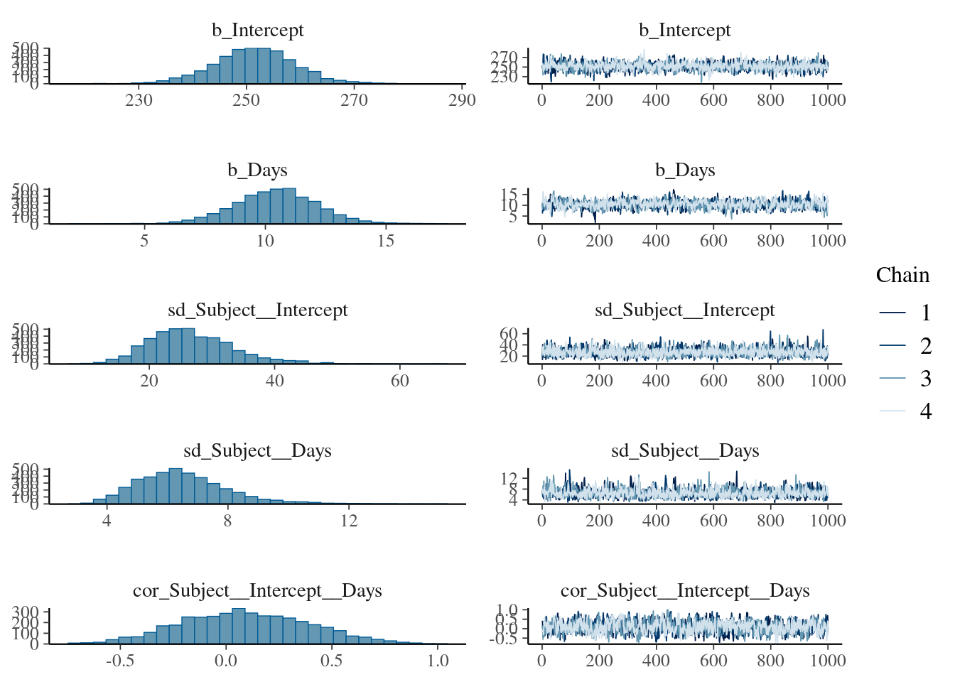
For convergence, Rhat values should not be above 1.00.

Code

summary(fit_sleep3)

 Family: gaussian 
  Links: mu = identity 
Formula: Reaction ~ 1 + Days + (1 + Days | Subject) 
   Data: sleepstudy (Number of observations: 180) 
  Draws: 4 chains, each with iter = 2000; warmup = 1000; thin = 1;
         total post-warmup draws = 4000

Multilevel Hyperparameters:
~Subject (Number of levels: 18) 
                    Estimate Est.Error l-95% CI u-95% CI Rhat Bulk_ESS Tail_ESS
sd(Intercept)          26.76      6.70    15.60    41.96 1.00     1836     2290
sd(Days)                6.58      1.55     4.17    10.23 1.00     1265     1938
cor(Intercept,Days)     0.08      0.30    -0.49     0.66 1.00     1041     1736

Regression Coefficients:
          Estimate Est.Error l-95% CI u-95% CI Rhat Bulk_ESS Tail_ESS
Intercept   251.38      7.39   236.80   266.10 1.00     1912     2086
Days         10.43      1.76     7.03    13.97 1.00     1294     1865

Further Distributional Parameters:
      Estimate Est.Error l-95% CI u-95% CI Rhat Bulk_ESS Tail_ESS
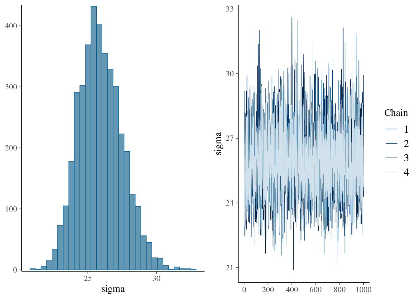
sigma    25.96      1.55    23.13    29.23 1.00     3535     2807

Draws were sampled using sampling(NUTS). For each parameter, Bulk_ESS
and Tail_ESS are effective sample size measures, and Rhat is the potential
scale reduction factor on split chains (at convergence, Rhat = 1).

3.3 Model Priors

Code

prior_summary(fit_sleep3)

3.4 Model Parameters

Code

variables(fit_sleep3)

 [1] "b_Intercept"                  "b_Days"                      
 [3] "sd_Subject__Intercept"        "sd_Subject__Days"            
 [5] "cor_Subject__Intercept__Days" "sigma"                       
 [7] "Intercept"                    "r_Subject[308,Intercept]"    
 [9] "r_Subject[309,Intercept]"     "r_Subject[310,Intercept]"    
[11] "r_Subject[330,Intercept]"     "r_Subject[331,Intercept]"    
[13] "r_Subject[332,Intercept]"     "r_Subject[333,Intercept]"    
[15] "r_Subject[334,Intercept]"     "r_Subject[335,Intercept]"    
[17] "r_Subject[337,Intercept]"     "r_Subject[349,Intercept]"    
[19] "r_Subject[350,Intercept]"     "r_Subject[351,Intercept]"    
[21] "r_Subject[352,Intercept]"     "r_Subject[369,Intercept]"    
[23] "r_Subject[370,Intercept]"     "r_Subject[371,Intercept]"    
[25] "r_Subject[372,Intercept]"     "r_Subject[308,Days]"         
[27] "r_Subject[309,Days]"          "r_Subject[310,Days]"         
[29] "r_Subject[330,Days]"          "r_Subject[331,Days]"         
[31] "r_Subject[332,Days]"          "r_Subject[333,Days]"         
[33] "r_Subject[334,Days]"          "r_Subject[335,Days]"         
[35] "r_Subject[337,Days]"          "r_Subject[349,Days]"         
[37] "r_Subject[350,Days]"          "r_Subject[351,Days]"         
[39] "r_Subject[352,Days]"          "r_Subject[369,Days]"         
[41] "r_Subject[370,Days]"          "r_Subject[371,Days]"         
[43] "r_Subject[372,Days]"          "lprior"                      
[45] "lp__"

3.5 Model Coefficients

Code

coef(fit_sleep3)

$Subject
, , Intercept

    Estimate Est.Error     Q2.5    Q97.5
308 253.8036  13.42340 227.2528 279.4458
309 211.5798  13.53907 184.5701 237.5476
310 212.9776  13.44786 186.3989 238.6100
330 274.5239  13.43628 248.1815 301.9403
331 273.0398  13.23918 248.1694 299.4477
332 260.2840  12.23798 236.3152 284.9809
333 267.8093  12.62690 244.2342 293.6989
334 244.3311  12.62822 219.1096 269.0711
335 250.7611  13.16495 224.1951 276.3869
337 286.1682  13.38914 259.9519 312.2581
349 226.5570  12.82480 200.4294 251.4542
350 238.6786  13.13686 212.3307 263.6997
351 255.7790  12.53802 230.2905 280.3204
352 272.2132  12.54778 247.9377 297.7906
369 254.4293  12.50311 230.2014 278.3378
370 226.7179  13.30644 200.0374 251.3793
371 252.3647  12.07777 229.1029 275.8134
372 263.5458  12.38755 239.3714 287.7161

, , Days

      Estimate Est.Error        Q2.5     Q97.5
308 19.6319154  2.542400 14.91127989 24.921229
309  1.7458810  2.561539 -3.16997162  6.728358
310  4.9887767  2.536991  0.03313305 10.034349
330  5.7537881  2.555568  0.62257977 10.503648
331  7.5170261  2.469967  2.42232385 12.196072
332 10.2271380  2.325028  5.69008473 14.750818
333 10.2869556  2.337880  5.51782984 14.730549
334 11.5339766  2.405073  6.85791261 16.290102
335 -0.2252846  2.582433 -5.24670583  4.873086
337 19.1100826  2.537751 14.24044379 24.060945
349 11.5705306  2.403886  7.01645714 16.487190
350 17.0331885  2.543700 12.24508630 22.034614
351  7.4875668  2.395344  2.89592486 12.176265
352 14.0213129  2.421787  9.20693205 18.780621
369 11.3270352  2.379922  6.54155107 15.929727
370 15.1243321  2.534860 10.24501333 20.291155
371  9.4030963  2.306262  4.87040862 14.017797
372 11.7617904  2.361364  7.07438198 16.475036

3.6 Plots

3.6.1 Trace Plots

Code

plot(fit_sleep3, ask = FALSE)

3.6.2 Visualize Predictions

3.6.2.1 Sample-Level

Code

plot(conditional_effects(fit_sleep1), points = TRUE)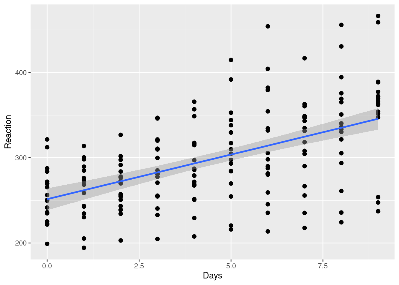

3.6.2.2 Person-Level

Code

# re_formula = NULL ensures that group-level effects are included
ce2 <- conditional_effects(
  fit_sleep3,
  conditions = conditions,
  re_formula = NULL)

plot(ce2, ncol = 6, points = TRUE)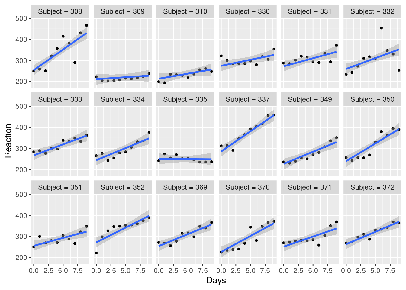

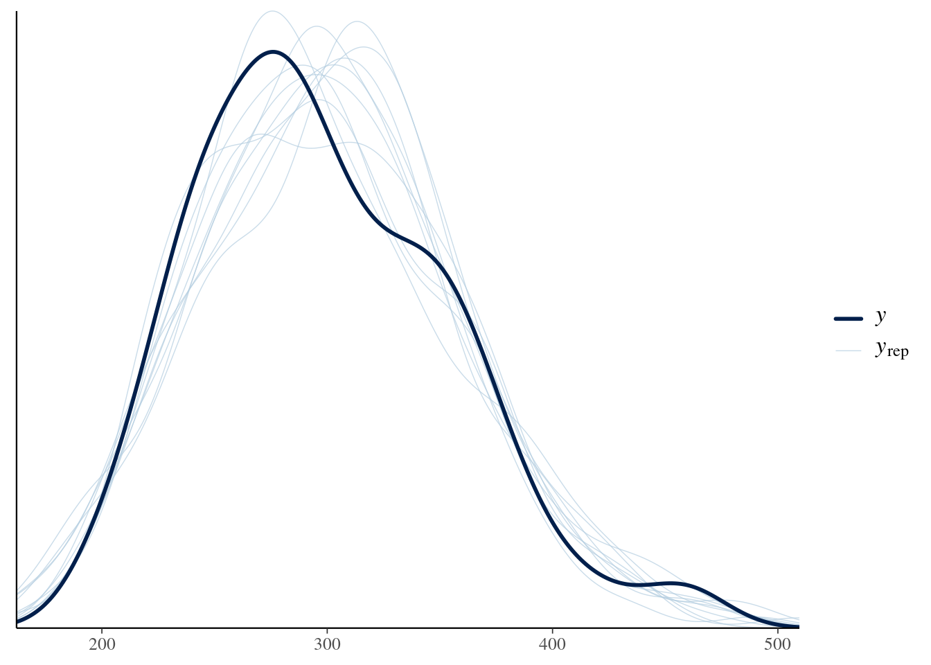
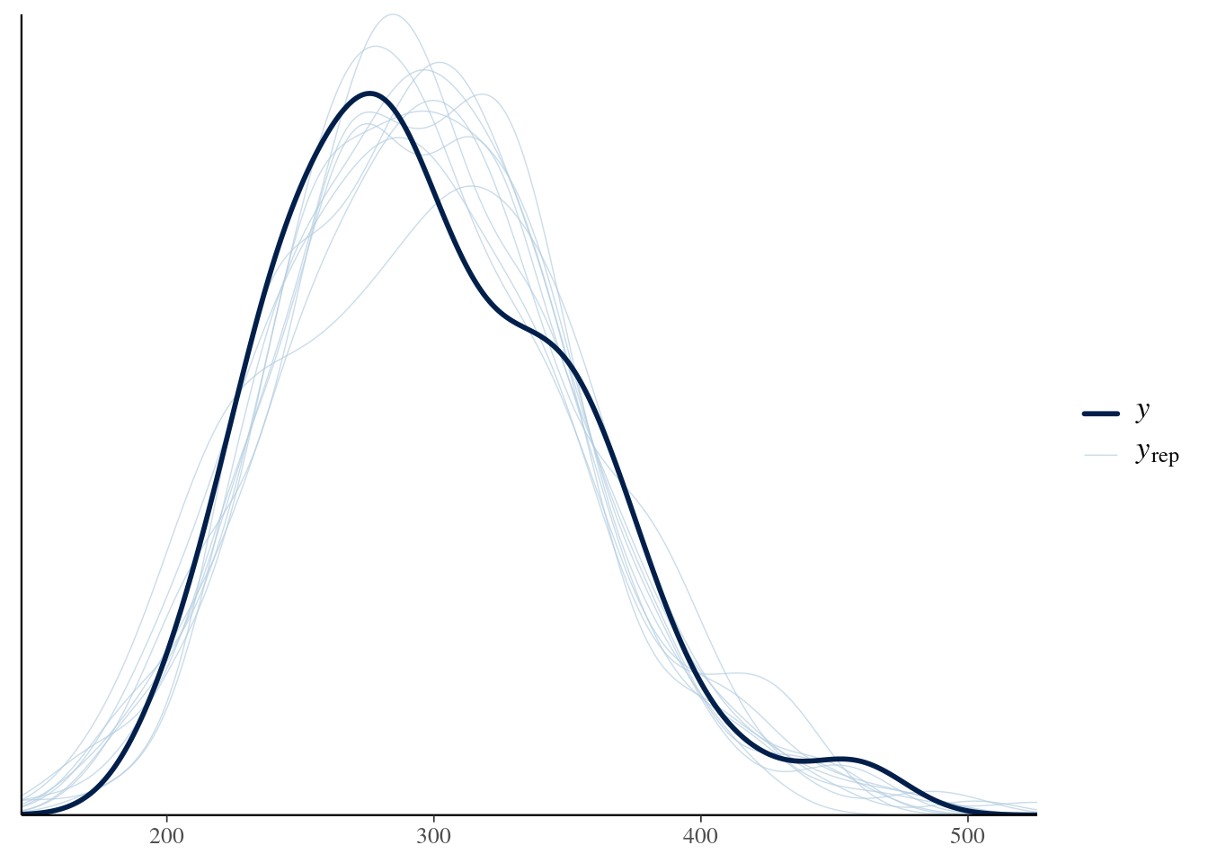
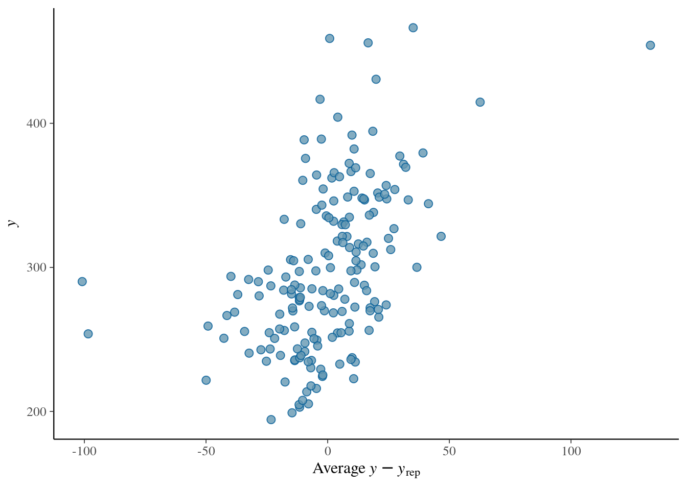
3.6.3 Check Model Fit

3.6.3.1 Posterior Predictive Check

Evaluate how closely the posterior predictions match the observed values. If they do not match the general pattern of the observed values, a different response distribution may be necessary.

Code

pp_check(fit_sleep3)

Code

pp_check(fit_sleep3, type = "dens_overlay")

Code

pp_check(fit_sleep3, "error_scatter_avg")

3.7 Fitted Values

Code

fitted(fit_sleep3)

     Estimate Est.Error     Q2.5    Q97.5
[1,] 253.8036 13.423405 227.2528 279.4458
[2,] 273.4355 11.520427 251.1066 295.5886
[3,] 293.0674  9.908596 273.5416 312.1998
[4,] 312.6994  8.750308 295.6254 329.6635
[5,] 332.3313  8.239121 316.1146 348.5817
[6,] 351.9632  8.492698 335.3675 368.3632

3.8 Residuals

Code

residuals(fit_sleep3)

       Estimate Est.Error       Q2.5     Q97.5
[1,]  -4.359981  29.46692 -61.815395  53.49204
[2,] -14.933307  27.93148 -69.475757  40.72256
[3,] -42.789309  27.97917 -98.036432  11.56407
[4,]   8.919060  26.99970 -44.082283  62.02641
[5,]  24.730870  26.95023 -28.225305  78.96176
[6,]  62.923941  27.86174   8.663845 117.81347

3.9 Compare Models

elpd values: higher is better looic values: lower is better

elpd_diff values that are greater than ~2 standard errors of the elpd_diff values indicate a significantly better model (i.e., if elpd_diff value is greater than 2 times the se_diff value).

Code

loo(fit_sleep1, fit_sleep2, fit_sleep3)

Output of model 'fit_sleep1':

Computed from 4000 by 180 log-likelihood matrix.

         Estimate   SE
elpd_loo   -953.1 10.5
p_loo         3.0  0.5
looic      1906.3 21.0
------
MCSE of elpd_loo is 0.0.
MCSE and ESS estimates assume MCMC draws (r_eff in [0.9, 1.2]).

All Pareto k estimates are good (k < 0.7).
See help('pareto-k-diagnostic') for details.

Output of model 'fit_sleep2':

Computed from 4000 by 180 log-likelihood matrix.

         Estimate   SE
elpd_loo   -884.7 14.3
p_loo        19.2  3.3
looic      1769.4 28.7
------
MCSE of elpd_loo is 0.1.
MCSE and ESS estimates assume MCMC draws (r_eff in [0.4, 1.8]).

All Pareto k estimates are good (k < 0.7).
See help('pareto-k-diagnostic') for details.

Output of model 'fit_sleep3':

Computed from 4000 by 180 log-likelihood matrix.

         Estimate   SE
elpd_loo   -861.2 22.1
p_loo        34.0  8.2
looic      1722.4 44.1
------
MCSE of elpd_loo is NA.
MCSE and ESS estimates assume MCMC draws (r_eff in [0.5, 1.2]).

Pareto k diagnostic values:
                         Count Pct.    Min. ESS
(-Inf, 0.7]   (good)     177   98.3%   49      
   (0.7, 1]   (bad)        3    1.7%   <NA>    
   (1, Inf)   (very bad)   0    0.0%   <NA>    
See help('pareto-k-diagnostic') for details.

Model comparisons:
           elpd_diff se_diff
fit_sleep3   0.0       0.0  
fit_sleep2 -23.5      11.4  
fit_sleep1 -91.9      20.7

Code

print(loo(fit_sleep1, fit_sleep2, fit_sleep3), simplify = FALSE)

Output of model 'fit_sleep1':

Computed from 4000 by 180 log-likelihood matrix.

         Estimate   SE
elpd_loo   -953.1 10.5
p_loo         3.0  0.5
looic      1906.3 21.0
------
MCSE of elpd_loo is 0.0.
MCSE and ESS estimates assume MCMC draws (r_eff in [0.9, 1.2]).

All Pareto k estimates are good (k < 0.7).
See help('pareto-k-diagnostic') for details.

Output of model 'fit_sleep2':

Computed from 4000 by 180 log-likelihood matrix.

         Estimate   SE
elpd_loo   -884.7 14.3
p_loo        19.2  3.3
looic      1769.4 28.7
------
MCSE of elpd_loo is 0.1.
MCSE and ESS estimates assume MCMC draws (r_eff in [0.4, 1.8]).

All Pareto k estimates are good (k < 0.7).
See help('pareto-k-diagnostic') for details.

Output of model 'fit_sleep3':

Computed from 4000 by 180 log-likelihood matrix.

         Estimate   SE
elpd_loo   -861.2 22.1
p_loo        34.0  8.2
looic      1722.4 44.1
------
MCSE of elpd_loo is NA.
MCSE and ESS estimates assume MCMC draws (r_eff in [0.5, 1.2]).

Pareto k diagnostic values:
                         Count Pct.    Min. ESS
(-Inf, 0.7]   (good)     177   98.3%   49      
   (0.7, 1]   (bad)        3    1.7%   <NA>    
   (1, Inf)   (very bad)   0    0.0%   <NA>    
See help('pareto-k-diagnostic') for details.

Model comparisons:
           elpd_diff se_diff elpd_loo se_elpd_loo p_loo  se_p_loo looic 
fit_sleep3    0.0       0.0  -861.2     22.1        34.0    8.2   1722.4
fit_sleep2  -23.5      11.4  -884.7     14.3        19.2    3.3   1769.4
fit_sleep1  -91.9      20.7  -953.1     10.5         3.0    0.5   1906.3
           se_looic
fit_sleep3   44.1  
fit_sleep2   28.7  
fit_sleep1   21.0

3.9.1 Compute Model Weights

Code

model_weights(fit_sleep1, fit_sleep2, fit_sleep3, weights = "loo")

  fit_sleep1   fit_sleep2   fit_sleep3 
1.192945e-40 6.120337e-11 1.000000e+00

Code

round(model_weights(fit_sleep1, fit_sleep2, fit_sleep3, weights = "loo"))

fit_sleep1 fit_sleep2 fit_sleep3 
         0          0          1

4 Multilevel Mediation

The syntax below estimates random intercepts (which allows each participant to have a different intercept) to account for nested data within the same participant.

Code

bayesianMediationSyntax <-
  bf(M ~ X + (1 |i| id)) +
  bf(Y ~ X + M + (1 |i| id)) +
  set_rescor(FALSE) # don't add a residual correlation between M and Y

bayesianMediationModel <- brm(
  bayesianMediationSyntax,
  data  = mydata,
  seed  = 52242
)


SAMPLING FOR MODEL 'anon_model' NOW (CHAIN 1).
Chain 1: 
Chain 1: Gradient evaluation took 0.000134 seconds
Chain 1: 1000 transitions using 10 leapfrog steps per transition would take 1.34 seconds.
Chain 1: Adjust your expectations accordingly!
Chain 1: 
Chain 1: 
Chain 1: Iteration:    1 / 2000 [  0%]  (Warmup)
Chain 1: Iteration:  200 / 2000 [ 10%]  (Warmup)
Chain 1: Iteration:  400 / 2000 [ 20%]  (Warmup)
Chain 1: Iteration:  600 / 2000 [ 30%]  (Warmup)
Chain 1: Iteration:  800 / 2000 [ 40%]  (Warmup)
Chain 1: Iteration: 1000 / 2000 [ 50%]  (Warmup)
Chain 1: Iteration: 1001 / 2000 [ 50%]  (Sampling)
Chain 1: Iteration: 1200 / 2000 [ 60%]  (Sampling)
Chain 1: Iteration: 1400 / 2000 [ 70%]  (Sampling)
Chain 1: Iteration: 1600 / 2000 [ 80%]  (Sampling)
Chain 1: Iteration: 1800 / 2000 [ 90%]  (Sampling)
Chain 1: Iteration: 2000 / 2000 [100%]  (Sampling)
Chain 1: 
Chain 1:  Elapsed Time: 5.287 seconds (Warm-up)
Chain 1:                3.508 seconds (Sampling)
Chain 1:                8.795 seconds (Total)
Chain 1: 

SAMPLING FOR MODEL 'anon_model' NOW (CHAIN 2).
Chain 2: 
Chain 2: Gradient evaluation took 0.000109 seconds
Chain 2: 1000 transitions using 10 leapfrog steps per transition would take 1.09 seconds.
Chain 2: Adjust your expectations accordingly!
Chain 2: 
Chain 2: 
Chain 2: Iteration:    1 / 2000 [  0%]  (Warmup)
Chain 2: Iteration:  200 / 2000 [ 10%]  (Warmup)
Chain 2: Iteration:  400 / 2000 [ 20%]  (Warmup)
Chain 2: Iteration:  600 / 2000 [ 30%]  (Warmup)
Chain 2: Iteration:  800 / 2000 [ 40%]  (Warmup)
Chain 2: Iteration: 1000 / 2000 [ 50%]  (Warmup)
Chain 2: Iteration: 1001 / 2000 [ 50%]  (Sampling)
Chain 2: Iteration: 1200 / 2000 [ 60%]  (Sampling)
Chain 2: Iteration: 1400 / 2000 [ 70%]  (Sampling)
Chain 2: Iteration: 1600 / 2000 [ 80%]  (Sampling)
Chain 2: Iteration: 1800 / 2000 [ 90%]  (Sampling)
Chain 2: Iteration: 2000 / 2000 [100%]  (Sampling)
Chain 2: 
Chain 2:  Elapsed Time: 5.113 seconds (Warm-up)
Chain 2:                3.389 seconds (Sampling)
Chain 2:                8.502 seconds (Total)
Chain 2: 

SAMPLING FOR MODEL 'anon_model' NOW (CHAIN 3).
Chain 3: 
Chain 3: Gradient evaluation took 0.000112 seconds
Chain 3: 1000 transitions using 10 leapfrog steps per transition would take 1.12 seconds.
Chain 3: Adjust your expectations accordingly!
Chain 3: 
Chain 3: 
Chain 3: Iteration:    1 / 2000 [  0%]  (Warmup)
Chain 3: Iteration:  200 / 2000 [ 10%]  (Warmup)
Chain 3: Iteration:  400 / 2000 [ 20%]  (Warmup)
Chain 3: Iteration:  600 / 2000 [ 30%]  (Warmup)
Chain 3: Iteration:  800 / 2000 [ 40%]  (Warmup)
Chain 3: Iteration: 1000 / 2000 [ 50%]  (Warmup)
Chain 3: Iteration: 1001 / 2000 [ 50%]  (Sampling)
Chain 3: Iteration: 1200 / 2000 [ 60%]  (Sampling)
Chain 3: Iteration: 1400 / 2000 [ 70%]  (Sampling)
Chain 3: Iteration: 1600 / 2000 [ 80%]  (Sampling)
Chain 3: Iteration: 1800 / 2000 [ 90%]  (Sampling)
Chain 3: Iteration: 2000 / 2000 [100%]  (Sampling)
Chain 3: 
Chain 3:  Elapsed Time: 5.07 seconds (Warm-up)
Chain 3:                3.509 seconds (Sampling)
Chain 3:                8.579 seconds (Total)
Chain 3: 

SAMPLING FOR MODEL 'anon_model' NOW (CHAIN 4).
Chain 4: 
Chain 4: Gradient evaluation took 0.000126 seconds
Chain 4: 1000 transitions using 10 leapfrog steps per transition would take 1.26 seconds.
Chain 4: Adjust your expectations accordingly!
Chain 4: 
Chain 4: 
Chain 4: Iteration:    1 / 2000 [  0%]  (Warmup)
Chain 4: Iteration:  200 / 2000 [ 10%]  (Warmup)
Chain 4: Iteration:  400 / 2000 [ 20%]  (Warmup)
Chain 4: Iteration:  600 / 2000 [ 30%]  (Warmup)
Chain 4: Iteration:  800 / 2000 [ 40%]  (Warmup)
Chain 4: Iteration: 1000 / 2000 [ 50%]  (Warmup)
Chain 4: Iteration: 1001 / 2000 [ 50%]  (Sampling)
Chain 4: Iteration: 1200 / 2000 [ 60%]  (Sampling)
Chain 4: Iteration: 1400 / 2000 [ 70%]  (Sampling)
Chain 4: Iteration: 1600 / 2000 [ 80%]  (Sampling)
Chain 4: Iteration: 1800 / 2000 [ 90%]  (Sampling)
Chain 4: Iteration: 2000 / 2000 [100%]  (Sampling)
Chain 4: 
Chain 4:  Elapsed Time: 4.877 seconds (Warm-up)
Chain 4:                2.834 seconds (Sampling)
Chain 4:                7.711 seconds (Total)
Chain 4:

Code

summary(bayesianMediationModel)

 Family: MV(gaussian, gaussian) 
  Links: mu = identity
         mu = identity 
Formula: M ~ X + (1 | i | id) 
         Y ~ X + M + (1 | i | id) 
   Data: mydata (Number of observations: 970) 
  Draws: 4 chains, each with iter = 2000; warmup = 1000; thin = 1;
         total post-warmup draws = 4000

Multilevel Hyperparameters:
~id (Number of levels: 100) 
                             Estimate Est.Error l-95% CI u-95% CI Rhat Bulk_ESS
sd(M_Intercept)                  0.07      0.05     0.00     0.17 1.00     1697
sd(Y_Intercept)                  0.11      0.06     0.01     0.23 1.00     1061
cor(M_Intercept,Y_Intercept)     0.04      0.55    -0.93     0.95 1.00     1275
                             Tail_ESS
sd(M_Intercept)                  2298
sd(Y_Intercept)                  1675
cor(M_Intercept,Y_Intercept)     1906

Regression Coefficients:
            Estimate Est.Error l-95% CI u-95% CI Rhat Bulk_ESS Tail_ESS
M_Intercept     0.00      0.03    -0.06     0.07 1.00     6932     3140
Y_Intercept     0.06      0.03    -0.01     0.13 1.00     6151     2914
M_X             0.51      0.03     0.44     0.58 1.00     7856     2892
Y_X             0.03      0.04    -0.04     0.10 1.00     6309     3423
Y_M             0.68      0.03     0.62     0.75 1.00     6429     3024

Further Distributional Parameters:
        Estimate Est.Error l-95% CI u-95% CI Rhat Bulk_ESS Tail_ESS
sigma_M     1.01      0.02     0.97     1.06 1.00     6987     1902
sigma_Y     1.00      0.02     0.96     1.05 1.00     4782     2966

Draws were sampled using sampling(NUTS). For each parameter, Bulk_ESS
and Tail_ESS are effective sample size measures, and Rhat is the potential
scale reduction factor on split chains (at convergence, Rhat = 1).

Code

hypothesis(
  bayesianMediationModel,
  "b_M_X * b_Y_M = 0", # indirect effect = a path * b path
  class = NULL,
  seed  =  52242
)

Hypothesis Tests for class :
         Hypothesis Estimate Est.Error CI.Lower CI.Upper Evid.Ratio Post.Prob
1 (b_M_X*b_Y_M) = 0     0.35      0.03     0.29      0.4         NA        NA
  Star
1    *
---
'CI': 90%-CI for one-sided and 95%-CI for two-sided hypotheses.
'*': For one-sided hypotheses, the posterior probability exceeds 95%;
for two-sided hypotheses, the value tested against lies outside the 95%-CI.
Posterior probabilities of point hypotheses assume equal prior probabilities.

Code

mediation(bayesianMediationModel)

5 Setting Priors

5.1 Parameters for Which to Set Priors

Code

get_prior(
  Reaction ~ 1 + Days + (1 + Days | Subject), 
  data = sleepstudy)

5.2 Define Priors

Code

bprior <- c(
  set_prior("normal(5, 5)", coef = "Days"),
  set_prior("cauchy(0, 10)", class = "sd"),
  set_prior("lkj(2)", class = "cor"))

bprior

5.3 Fit the Model

Fit the model with these priors, and sample from these priors:

Code

fit_sleep4 <- brm(
  Reaction ~ 1 + Days + (1 + Days | Subject), 
  data = sleepstudy,
  prior = bprior, 
  sample_prior = TRUE,
  seed  = 52242
)

6 Evaluate a Hypothesis

Code

# Evid.Ratio is the ratio of P(Days > 7) / P(Days <= 7)
(hyp1 <- hypothesis(fit_sleep4, "Days < 7"))

Hypothesis Tests for class b:
      Hypothesis Estimate Est.Error CI.Lower CI.Upper Evid.Ratio Post.Prob Star
1 (Days)-(7) < 0     2.84      1.59     0.18      5.4       0.04      0.04     
---
'CI': 90%-CI for one-sided and 95%-CI for two-sided hypotheses.
'*': For one-sided hypotheses, the posterior probability exceeds 95%;
for two-sided hypotheses, the value tested against lies outside the 95%-CI.
Posterior probabilities of point hypotheses assume equal prior probabilities.

Code

plot(hyp1)

Code

# Evid.Ratio is the Bayes Factor of the posterior
# vs the prior that Days = 10 is TRUE (Savage-Dickey Ratio)
(hyp2 <- hypothesis(fit_sleep4, "Days = 10"))

Hypothesis Tests for class b:
       Hypothesis Estimate Est.Error CI.Lower CI.Upper Evid.Ratio Post.Prob
1 (Days)-(10) = 0    -0.16      1.59    -3.32     2.75       5.17      0.84
  Star
1     
---
'CI': 90%-CI for one-sided and 95%-CI for two-sided hypotheses.
'*': For one-sided hypotheses, the posterior probability exceeds 95%;
for two-sided hypotheses, the value tested against lies outside the 95%-CI.
Posterior probabilities of point hypotheses assume equal prior probabilities.

Code

plot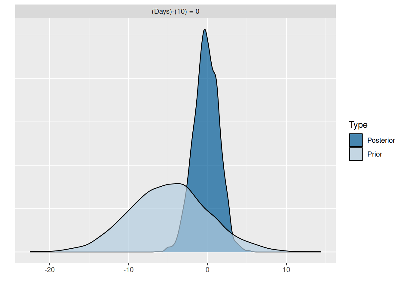(hyp2)

7 Parallel Processing

7.1 Between-Chain Parallelization

Code

fit_sleep4 <- brm(
  Reaction ~ 1 + Days + (1 + Days | Subject), 
  data = sleepstudy,
  prior = bprior, 
  sample_prior = TRUE,
  cores = 4,
  seed  = 52242
)

7.2 Within-Chain Parallelization

https://paul-buerkner.github.io/brms/articles/brms_threading.html (archived at https://perma.cc/NCG3-KV4G)

8 Missing Data Handling

8.1 Multiply Imputed Datasets from `mice`

Code

?brm_multiple

Code

imp <- mice::mice(
  mydata,
  m = 5,
  print = FALSE)

fit_imp <- brm_multiple(
  bayesianMediationSyntax,
  data = imp,
  chains = 2)


SAMPLING FOR MODEL 'anon_model' NOW (CHAIN 1).
Chain 1: 
Chain 1: Gradient evaluation took 0.000356 seconds
Chain 1: 1000 transitions using 10 leapfrog steps per transition would take 3.56 seconds.
Chain 1: Adjust your expectations accordingly!
Chain 1: 
Chain 1: 
Chain 1: Iteration:    1 / 2000 [  0%]  (Warmup)
Chain 1: Iteration:  200 / 2000 [ 10%]  (Warmup)
Chain 1: Iteration:  400 / 2000 [ 20%]  (Warmup)
Chain 1: Iteration:  600 / 2000 [ 30%]  (Warmup)
Chain 1: Iteration:  800 / 2000 [ 40%]  (Warmup)
Chain 1: Iteration: 1000 / 2000 [ 50%]  (Warmup)
Chain 1: Iteration: 1001 / 2000 [ 50%]  (Sampling)
Chain 1: Iteration: 1200 / 2000 [ 60%]  (Sampling)
Chain 1: Iteration: 1400 / 2000 [ 70%]  (Sampling)
Chain 1: Iteration: 1600 / 2000 [ 80%]  (Sampling)
Chain 1: Iteration: 1800 / 2000 [ 90%]  (Sampling)
Chain 1: Iteration: 2000 / 2000 [100%]  (Sampling)
Chain 1: 
Chain 1:  Elapsed Time: 4.747 seconds (Warm-up)
Chain 1:                2.487 seconds (Sampling)
Chain 1:                7.234 seconds (Total)
Chain 1: 

SAMPLING FOR MODEL 'anon_model' NOW (CHAIN 2).
Chain 2: 
Chain 2: Gradient evaluation took 0.000114 seconds
Chain 2: 1000 transitions using 10 leapfrog steps per transition would take 1.14 seconds.
Chain 2: Adjust your expectations accordingly!
Chain 2: 
Chain 2: 
Chain 2: Iteration:    1 / 2000 [  0%]  (Warmup)
Chain 2: Iteration:  200 / 2000 [ 10%]  (Warmup)
Chain 2: Iteration:  400 / 2000 [ 20%]  (Warmup)
Chain 2: Iteration:  600 / 2000 [ 30%]  (Warmup)
Chain 2: Iteration:  800 / 2000 [ 40%]  (Warmup)
Chain 2: Iteration: 1000 / 2000 [ 50%]  (Warmup)
Chain 2: Iteration: 1001 / 2000 [ 50%]  (Sampling)
Chain 2: Iteration: 1200 / 2000 [ 60%]  (Sampling)
Chain 2: Iteration: 1400 / 2000 [ 70%]  (Sampling)
Chain 2: Iteration: 1600 / 2000 [ 80%]  (Sampling)
Chain 2: Iteration: 1800 / 2000 [ 90%]  (Sampling)
Chain 2: Iteration: 2000 / 2000 [100%]  (Sampling)
Chain 2: 
Chain 2:  Elapsed Time: 5.286 seconds (Warm-up)
Chain 2:                2.482 seconds (Sampling)
Chain 2:                7.768 seconds (Total)
Chain 2: 

SAMPLING FOR MODEL 'anon_model' NOW (CHAIN 1).
Chain 1: 
Chain 1: Gradient evaluation took 0.000129 seconds
Chain 1: 1000 transitions using 10 leapfrog steps per transition would take 1.29 seconds.
Chain 1: Adjust your expectations accordingly!
Chain 1: 
Chain 1: 
Chain 1: Iteration:    1 / 2000 [  0%]  (Warmup)
Chain 1: Iteration:  200 / 2000 [ 10%]  (Warmup)
Chain 1: Iteration:  400 / 2000 [ 20%]  (Warmup)
Chain 1: Iteration:  600 / 2000 [ 30%]  (Warmup)
Chain 1: Iteration:  800 / 2000 [ 40%]  (Warmup)
Chain 1: Iteration: 1000 / 2000 [ 50%]  (Warmup)
Chain 1: Iteration: 1001 / 2000 [ 50%]  (Sampling)
Chain 1: Iteration: 1200 / 2000 [ 60%]  (Sampling)
Chain 1: Iteration: 1400 / 2000 [ 70%]  (Sampling)
Chain 1: Iteration: 1600 / 2000 [ 80%]  (Sampling)
Chain 1: Iteration: 1800 / 2000 [ 90%]  (Sampling)
Chain 1: Iteration: 2000 / 2000 [100%]  (Sampling)
Chain 1: 
Chain 1:  Elapsed Time: 5.358 seconds (Warm-up)
Chain 1:                3.663 seconds (Sampling)
Chain 1:                9.021 seconds (Total)
Chain 1: 

SAMPLING FOR MODEL 'anon_model' NOW (CHAIN 2).
Chain 2: 
Chain 2: Gradient evaluation took 0.000115 seconds
Chain 2: 1000 transitions using 10 leapfrog steps per transition would take 1.15 seconds.
Chain 2: Adjust your expectations accordingly!
Chain 2: 
Chain 2: 
Chain 2: Iteration:    1 / 2000 [  0%]  (Warmup)
Chain 2: Iteration:  200 / 2000 [ 10%]  (Warmup)
Chain 2: Iteration:  400 / 2000 [ 20%]  (Warmup)
Chain 2: Iteration:  600 / 2000 [ 30%]  (Warmup)
Chain 2: Iteration:  800 / 2000 [ 40%]  (Warmup)
Chain 2: Iteration: 1000 / 2000 [ 50%]  (Warmup)
Chain 2: Iteration: 1001 / 2000 [ 50%]  (Sampling)
Chain 2: Iteration: 1200 / 2000 [ 60%]  (Sampling)
Chain 2: Iteration: 1400 / 2000 [ 70%]  (Sampling)
Chain 2: Iteration: 1600 / 2000 [ 80%]  (Sampling)
Chain 2: Iteration: 1800 / 2000 [ 90%]  (Sampling)
Chain 2: Iteration: 2000 / 2000 [100%]  (Sampling)
Chain 2: 
Chain 2:  Elapsed Time: 5.597 seconds (Warm-up)
Chain 2:                1.84 seconds (Sampling)
Chain 2:                7.437 seconds (Total)
Chain 2: 

SAMPLING FOR MODEL 'anon_model' NOW (CHAIN 1).
Chain 1: 
Chain 1: Gradient evaluation took 0.000122 seconds
Chain 1: 1000 transitions using 10 leapfrog steps per transition would take 1.22 seconds.
Chain 1: Adjust your expectations accordingly!
Chain 1: 
Chain 1: 
Chain 1: Iteration:    1 / 2000 [  0%]  (Warmup)
Chain 1: Iteration:  200 / 2000 [ 10%]  (Warmup)
Chain 1: Iteration:  400 / 2000 [ 20%]  (Warmup)
Chain 1: Iteration:  600 / 2000 [ 30%]  (Warmup)
Chain 1: Iteration:  800 / 2000 [ 40%]  (Warmup)
Chain 1: Iteration: 1000 / 2000 [ 50%]  (Warmup)
Chain 1: Iteration: 1001 / 2000 [ 50%]  (Sampling)
Chain 1: Iteration: 1200 / 2000 [ 60%]  (Sampling)
Chain 1: Iteration: 1400 / 2000 [ 70%]  (Sampling)
Chain 1: Iteration: 1600 / 2000 [ 80%]  (Sampling)
Chain 1: Iteration: 1800 / 2000 [ 90%]  (Sampling)
Chain 1: Iteration: 2000 / 2000 [100%]  (Sampling)
Chain 1: 
Chain 1:  Elapsed Time: 5.017 seconds (Warm-up)
Chain 1:                3.58 seconds (Sampling)
Chain 1:                8.597 seconds (Total)
Chain 1: 

SAMPLING FOR MODEL 'anon_model' NOW (CHAIN 2).
Chain 2: 
Chain 2: Gradient evaluation took 0.000115 seconds
Chain 2: 1000 transitions using 10 leapfrog steps per transition would take 1.15 seconds.
Chain 2: Adjust your expectations accordingly!
Chain 2: 
Chain 2: 
Chain 2: Iteration:    1 / 2000 [  0%]  (Warmup)
Chain 2: Iteration:  200 / 2000 [ 10%]  (Warmup)
Chain 2: Iteration:  400 / 2000 [ 20%]  (Warmup)
Chain 2: Iteration:  600 / 2000 [ 30%]  (Warmup)
Chain 2: Iteration:  800 / 2000 [ 40%]  (Warmup)
Chain 2: Iteration: 1000 / 2000 [ 50%]  (Warmup)
Chain 2: Iteration: 1001 / 2000 [ 50%]  (Sampling)
Chain 2: Iteration: 1200 / 2000 [ 60%]  (Sampling)
Chain 2: Iteration: 1400 / 2000 [ 70%]  (Sampling)
Chain 2: Iteration: 1600 / 2000 [ 80%]  (Sampling)
Chain 2: Iteration: 1800 / 2000 [ 90%]  (Sampling)
Chain 2: Iteration: 2000 / 2000 [100%]  (Sampling)
Chain 2: 
Chain 2:  Elapsed Time: 5.148 seconds (Warm-up)
Chain 2:                3.644 seconds (Sampling)
Chain 2:                8.792 seconds (Total)
Chain 2: 

SAMPLING FOR MODEL 'anon_model' NOW (CHAIN 1).
Chain 1: 
Chain 1: Gradient evaluation took 0.000125 seconds
Chain 1: 1000 transitions using 10 leapfrog steps per transition would take 1.25 seconds.
Chain 1: Adjust your expectations accordingly!
Chain 1: 
Chain 1: 
Chain 1: Iteration:    1 / 2000 [  0%]  (Warmup)
Chain 1: Iteration:  200 / 2000 [ 10%]  (Warmup)
Chain 1: Iteration:  400 / 2000 [ 20%]  (Warmup)
Chain 1: Iteration:  600 / 2000 [ 30%]  (Warmup)
Chain 1: Iteration:  800 / 2000 [ 40%]  (Warmup)
Chain 1: Iteration: 1000 / 2000 [ 50%]  (Warmup)
Chain 1: Iteration: 1001 / 2000 [ 50%]  (Sampling)
Chain 1: Iteration: 1200 / 2000 [ 60%]  (Sampling)
Chain 1: Iteration: 1400 / 2000 [ 70%]  (Sampling)
Chain 1: Iteration: 1600 / 2000 [ 80%]  (Sampling)
Chain 1: Iteration: 1800 / 2000 [ 90%]  (Sampling)
Chain 1: Iteration: 2000 / 2000 [100%]  (Sampling)
Chain 1: 
Chain 1:  Elapsed Time: 5.049 seconds (Warm-up)
Chain 1:                3.547 seconds (Sampling)
Chain 1:                8.596 seconds (Total)
Chain 1: 

SAMPLING FOR MODEL 'anon_model' NOW (CHAIN 2).
Chain 2: 
Chain 2: Gradient evaluation took 0.000115 seconds
Chain 2: 1000 transitions using 10 leapfrog steps per transition would take 1.15 seconds.
Chain 2: Adjust your expectations accordingly!
Chain 2: 
Chain 2: 
Chain 2: Iteration:    1 / 2000 [  0%]  (Warmup)
Chain 2: Iteration:  200 / 2000 [ 10%]  (Warmup)
Chain 2: Iteration:  400 / 2000 [ 20%]  (Warmup)
Chain 2: Iteration:  600 / 2000 [ 30%]  (Warmup)
Chain 2: Iteration:  800 / 2000 [ 40%]  (Warmup)
Chain 2: Iteration: 1000 / 2000 [ 50%]  (Warmup)
Chain 2: Iteration: 1001 / 2000 [ 50%]  (Sampling)
Chain 2: Iteration: 1200 / 2000 [ 60%]  (Sampling)
Chain 2: Iteration: 1400 / 2000 [ 70%]  (Sampling)
Chain 2: Iteration: 1600 / 2000 [ 80%]  (Sampling)
Chain 2: Iteration: 1800 / 2000 [ 90%]  (Sampling)
Chain 2: Iteration: 2000 / 2000 [100%]  (Sampling)
Chain 2: 
Chain 2:  Elapsed Time: 4.673 seconds (Warm-up)
Chain 2:                2.189 seconds (Sampling)
Chain 2:                6.862 seconds (Total)
Chain 2: 

SAMPLING FOR MODEL 'anon_model' NOW (CHAIN 1).
Chain 1: 
Chain 1: Gradient evaluation took 0.000124 seconds
Chain 1: 1000 transitions using 10 leapfrog steps per transition would take 1.24 seconds.
Chain 1: Adjust your expectations accordingly!
Chain 1: 
Chain 1: 
Chain 1: Iteration:    1 / 2000 [  0%]  (Warmup)
Chain 1: Iteration:  200 / 2000 [ 10%]  (Warmup)
Chain 1: Iteration:  400 / 2000 [ 20%]  (Warmup)
Chain 1: Iteration:  600 / 2000 [ 30%]  (Warmup)
Chain 1: Iteration:  800 / 2000 [ 40%]  (Warmup)
Chain 1: Iteration: 1000 / 2000 [ 50%]  (Warmup)
Chain 1: Iteration: 1001 / 2000 [ 50%]  (Sampling)
Chain 1: Iteration: 1200 / 2000 [ 60%]  (Sampling)
Chain 1: Iteration: 1400 / 2000 [ 70%]  (Sampling)
Chain 1: Iteration: 1600 / 2000 [ 80%]  (Sampling)
Chain 1: Iteration: 1800 / 2000 [ 90%]  (Sampling)
Chain 1: Iteration: 2000 / 2000 [100%]  (Sampling)
Chain 1: 
Chain 1:  Elapsed Time: 4.749 seconds (Warm-up)
Chain 1:                3.644 seconds (Sampling)
Chain 1:                8.393 seconds (Total)
Chain 1: 

SAMPLING FOR MODEL 'anon_model' NOW (CHAIN 2).
Chain 2: 
Chain 2: Gradient evaluation took 0.000114 seconds
Chain 2: 1000 transitions using 10 leapfrog steps per transition would take 1.14 seconds.
Chain 2: Adjust your expectations accordingly!
Chain 2: 
Chain 2: 
Chain 2: Iteration:    1 / 2000 [  0%]  (Warmup)
Chain 2: Iteration:  200 / 2000 [ 10%]  (Warmup)
Chain 2: Iteration:  400 / 2000 [ 20%]  (Warmup)
Chain 2: Iteration:  600 / 2000 [ 30%]  (Warmup)
Chain 2: Iteration:  800 / 2000 [ 40%]  (Warmup)
Chain 2: Iteration: 1000 / 2000 [ 50%]  (Warmup)
Chain 2: Iteration: 1001 / 2000 [ 50%]  (Sampling)
Chain 2: Iteration: 1200 / 2000 [ 60%]  (Sampling)
Chain 2: Iteration: 1400 / 2000 [ 70%]  (Sampling)
Chain 2: Iteration: 1600 / 2000 [ 80%]  (Sampling)
Chain 2: Iteration: 1800 / 2000 [ 90%]  (Sampling)
Chain 2: Iteration: 2000 / 2000 [100%]  (Sampling)
Chain 2: 
Chain 2:  Elapsed Time: 4.798 seconds (Warm-up)
Chain 2:                3.645 seconds (Sampling)
Chain 2:                8.443 seconds (Total)
Chain 2:

8.2 Imputation on the Fly During Model Fitting

https://paul-buerkner.github.io/brms/articles/brms_missings.html (archived at https://perma.cc/4Y9L-USQR)

Code

?mi

Code

bayesianRegressionImputationSyntax <-
  bf(X | mi() ~ (1 |i| id)) +
  bf(M | mi() ~ mi(X) + (1 |i| id)) +
  bf(Y | mi() ~ mi(X) + mi(M) + (1 |i| id)) +
  set_rescor(FALSE) # don't add a residual correlation between X, M, and Y

bayesianRegressionModel <- brm(
  bayesianRegressionImputationSyntax,
  data = mydata,
  seed = 52242
)


SAMPLING FOR MODEL 'anon_model' NOW (CHAIN 1).
Chain 1: 
Chain 1: Gradient evaluation took 0.000592 seconds
Chain 1: 1000 transitions using 10 leapfrog steps per transition would take 5.92 seconds.
Chain 1: Adjust your expectations accordingly!
Chain 1: 
Chain 1: 
Chain 1: Iteration:    1 / 2000 [  0%]  (Warmup)
Chain 1: Iteration:  200 / 2000 [ 10%]  (Warmup)
Chain 1: Iteration:  400 / 2000 [ 20%]  (Warmup)
Chain 1: Iteration:  600 / 2000 [ 30%]  (Warmup)
Chain 1: Iteration:  800 / 2000 [ 40%]  (Warmup)
Chain 1: Iteration: 1000 / 2000 [ 50%]  (Warmup)
Chain 1: Iteration: 1001 / 2000 [ 50%]  (Sampling)
Chain 1: Iteration: 1200 / 2000 [ 60%]  (Sampling)
Chain 1: Iteration: 1400 / 2000 [ 70%]  (Sampling)
Chain 1: Iteration: 1600 / 2000 [ 80%]  (Sampling)
Chain 1: Iteration: 1800 / 2000 [ 90%]  (Sampling)
Chain 1: Iteration: 2000 / 2000 [100%]  (Sampling)
Chain 1: 
Chain 1:  Elapsed Time: 21.12 seconds (Warm-up)
Chain 1:                13.296 seconds (Sampling)
Chain 1:                34.416 seconds (Total)
Chain 1: 

SAMPLING FOR MODEL 'anon_model' NOW (CHAIN 2).
Chain 2: 
Chain 2: Gradient evaluation took 0.000413 seconds
Chain 2: 1000 transitions using 10 leapfrog steps per transition would take 4.13 seconds.
Chain 2: Adjust your expectations accordingly!
Chain 2: 
Chain 2: 
Chain 2: Iteration:    1 / 2000 [  0%]  (Warmup)
Chain 2: Iteration:  200 / 2000 [ 10%]  (Warmup)
Chain 2: Iteration:  400 / 2000 [ 20%]  (Warmup)
Chain 2: Iteration:  600 / 2000 [ 30%]  (Warmup)
Chain 2: Iteration:  800 / 2000 [ 40%]  (Warmup)
Chain 2: Iteration: 1000 / 2000 [ 50%]  (Warmup)
Chain 2: Iteration: 1001 / 2000 [ 50%]  (Sampling)
Chain 2: Iteration: 1200 / 2000 [ 60%]  (Sampling)
Chain 2: Iteration: 1400 / 2000 [ 70%]  (Sampling)
Chain 2: Iteration: 1600 / 2000 [ 80%]  (Sampling)
Chain 2: Iteration: 1800 / 2000 [ 90%]  (Sampling)
Chain 2: Iteration: 2000 / 2000 [100%]  (Sampling)
Chain 2: 
Chain 2:  Elapsed Time: 19.95 seconds (Warm-up)
Chain 2:                13.287 seconds (Sampling)
Chain 2:                33.237 seconds (Total)
Chain 2: 

SAMPLING FOR MODEL 'anon_model' NOW (CHAIN 3).
Chain 3: 
Chain 3: Gradient evaluation took 0.000417 seconds
Chain 3: 1000 transitions using 10 leapfrog steps per transition would take 4.17 seconds.
Chain 3: Adjust your expectations accordingly!
Chain 3: 
Chain 3: 
Chain 3: Iteration:    1 / 2000 [  0%]  (Warmup)
Chain 3: Iteration:  200 / 2000 [ 10%]  (Warmup)
Chain 3: Iteration:  400 / 2000 [ 20%]  (Warmup)
Chain 3: Iteration:  600 / 2000 [ 30%]  (Warmup)
Chain 3: Iteration:  800 / 2000 [ 40%]  (Warmup)
Chain 3: Iteration: 1000 / 2000 [ 50%]  (Warmup)
Chain 3: Iteration: 1001 / 2000 [ 50%]  (Sampling)
Chain 3: Iteration: 1200 / 2000 [ 60%]  (Sampling)
Chain 3: Iteration: 1400 / 2000 [ 70%]  (Sampling)
Chain 3: Iteration: 1600 / 2000 [ 80%]  (Sampling)
Chain 3: Iteration: 1800 / 2000 [ 90%]  (Sampling)
Chain 3: Iteration: 2000 / 2000 [100%]  (Sampling)
Chain 3: 
Chain 3:  Elapsed Time: 19.13 seconds (Warm-up)
Chain 3:                13.301 seconds (Sampling)
Chain 3:                32.431 seconds (Total)
Chain 3: 

SAMPLING FOR MODEL 'anon_model' NOW (CHAIN 4).
Chain 4: 
Chain 4: Gradient evaluation took 0.000414 seconds
Chain 4: 1000 transitions using 10 leapfrog steps per transition would take 4.14 seconds.
Chain 4: Adjust your expectations accordingly!
Chain 4: 
Chain 4: 
Chain 4: Iteration:    1 / 2000 [  0%]  (Warmup)
Chain 4: Iteration:  200 / 2000 [ 10%]  (Warmup)
Chain 4: Iteration:  400 / 2000 [ 20%]  (Warmup)
Chain 4: Iteration:  600 / 2000 [ 30%]  (Warmup)
Chain 4: Iteration:  800 / 2000 [ 40%]  (Warmup)
Chain 4: Iteration: 1000 / 2000 [ 50%]  (Warmup)
Chain 4: Iteration: 1001 / 2000 [ 50%]  (Sampling)
Chain 4: Iteration: 1200 / 2000 [ 60%]  (Sampling)
Chain 4: Iteration: 1400 / 2000 [ 70%]  (Sampling)
Chain 4: Iteration: 1600 / 2000 [ 80%]  (Sampling)
Chain 4: Iteration: 1800 / 2000 [ 90%]  (Sampling)
Chain 4: Iteration: 2000 / 2000 [100%]  (Sampling)
Chain 4: 
Chain 4:  Elapsed Time: 18.608 seconds (Warm-up)
Chain 4:                12.279 seconds (Sampling)
Chain 4:                30.887 seconds (Total)
Chain 4:

Code

summary(bayesianRegressionModel)

 Family: MV(gaussian, gaussian, gaussian) 
  Links: mu = identity
         mu = identity
         mu = identity 
Formula: X | mi() ~ (1 | i | id) 
         M | mi() ~ mi(X) + (1 | i | id) 
         Y | mi() ~ mi(X) + mi(M) + (1 | i | id) 
   Data: mydata (Number of observations: 1000) 
  Draws: 4 chains, each with iter = 2000; warmup = 1000; thin = 1;
         total post-warmup draws = 4000

Multilevel Hyperparameters:
~id (Number of levels: 100) 
                             Estimate Est.Error l-95% CI u-95% CI Rhat Bulk_ESS
sd(X_Intercept)                  0.09      0.06     0.00     0.21 1.00     1007
sd(M_Intercept)                  0.07      0.05     0.00     0.18 1.00     1534
sd(Y_Intercept)                  0.10      0.06     0.01     0.22 1.00     1310
cor(X_Intercept,M_Intercept)     0.08      0.49    -0.84     0.90 1.00     3556
cor(X_Intercept,Y_Intercept)     0.06      0.47    -0.82     0.88 1.00     2320
cor(M_Intercept,Y_Intercept)     0.00      0.48    -0.88     0.86 1.00     2474
                             Tail_ESS
sd(X_Intercept)                  1428
sd(M_Intercept)                  2177
sd(Y_Intercept)                  2087
cor(X_Intercept,M_Intercept)     2922
cor(X_Intercept,Y_Intercept)     2480
cor(M_Intercept,Y_Intercept)     2693

Regression Coefficients:
            Estimate Est.Error l-95% CI u-95% CI Rhat Bulk_ESS Tail_ESS
X_Intercept    -0.02      0.03    -0.08     0.05 1.00     7564     3001
M_Intercept     0.01      0.03    -0.06     0.07 1.00     7728     3049
Y_Intercept     0.06      0.03    -0.01     0.12 1.00     6781     2915
M_miX           0.51      0.03     0.45     0.58 1.00     8400     2801
Y_miX           0.04      0.04    -0.04     0.11 1.00     5567     2993
Y_miM           0.68      0.03     0.62     0.74 1.00     5954     3270

Further Distributional Parameters:
        Estimate Est.Error l-95% CI u-95% CI Rhat Bulk_ESS Tail_ESS
sigma_X     0.98      0.02     0.94     1.03 1.00     6184     2817
sigma_M     1.01      0.02     0.96     1.05 1.00     6661     2907
sigma_Y     1.01      0.02     0.96     1.05 1.00     5554     2605

Draws were sampled using sampling(NUTS). For each parameter, Bulk_ESS
and Tail_ESS are effective sample size measures, and Rhat is the potential
scale reduction factor on split chains (at convergence, Rhat = 1).

Code

hypothesis(
  bayesianRegressionModel,
  "bsp_M_miX * bsp_Y_miM = 0", # indirect effect = a path * b path
  class = NULL,
  seed = 52242
)

Hypothesis Tests for class :
                Hypothesis Estimate Est.Error CI.Lower CI.Upper Evid.Ratio
1 (bsp_M_miX*bsp_Y_... = 0     0.35      0.03      0.3      0.4         NA
  Post.Prob Star
1        NA    *
---
'CI': 90%-CI for one-sided and 95%-CI for two-sided hypotheses.
'*': For one-sided hypotheses, the posterior probability exceeds 95%;
for two-sided hypotheses, the value tested against lies outside the 95%-CI.
Posterior probabilities of point hypotheses assume equal prior probabilities.

9 Session Info

Code

sessionInfo()

R version 4.5.2 (2025-10-31)
Platform: x86_64-pc-linux-gnu
Running under: Ubuntu 24.04.3 LTS

Matrix products: default
BLAS:   /usr/lib/x86_64-linux-gnu/openblas-pthread/libblas.so.3 
LAPACK: /usr/lib/x86_64-linux-gnu/openblas-pthread/libopenblasp-r0.3.26.so;  LAPACK version 3.12.0

locale:
 [1] LC_CTYPE=C.UTF-8       LC_NUMERIC=C           LC_TIME=C.UTF-8       
 [4] LC_COLLATE=C.UTF-8     LC_MONETARY=C.UTF-8    LC_MESSAGES=C.UTF-8   
 [7] LC_PAPER=C.UTF-8       LC_NAME=C              LC_ADDRESS=C          
[10] LC_TELEPHONE=C         LC_MEASUREMENT=C.UTF-8 LC_IDENTIFICATION=C   

time zone: UTC
tzcode source: system (glibc)

attached base packages:
[1] stats     graphics  grDevices utils     datasets  methods   base     

other attached packages:
[1] future_1.68.0       mice_3.19.0         bayestestR_0.17.0  
[4] brms_2.23.0         Rcpp_1.1.0          rstan_2.32.7       
[7] StanHeaders_2.32.10 lme4_1.1-38         Matrix_1.7-4       

loaded via a namespace (and not attached):
 [1] tidyselect_1.2.1      dplyr_1.1.4           farver_2.1.2         
 [4] loo_2.9.0             S7_0.2.1              fastmap_1.2.0        
 [7] tensorA_0.36.2.1      digest_0.6.39         rpart_4.1.24         
[10] lifecycle_1.0.4       survival_3.8-3        processx_3.8.6       
[13] magrittr_2.0.4        posterior_1.6.1       compiler_4.5.2       
[16] rlang_1.1.6           tools_4.5.2           yaml_2.3.12          
[19] knitr_1.51            labeling_0.4.3        bridgesampling_1.2-1 
[22] htmlwidgets_1.6.4     pkgbuild_1.4.8        plyr_1.8.9           
[25] RColorBrewer_1.1-3    abind_1.4-8           withr_3.0.2          
[28] purrr_1.2.0           nnet_7.3-20           grid_4.5.2           
[31] stats4_4.5.2          jomo_2.7-6            inline_0.3.21        
[34] ggplot2_4.0.1         globals_0.18.0        scales_1.4.0         
[37] iterators_1.0.14      MASS_7.3-65           insight_1.4.4        
[40] cli_3.6.5             mvtnorm_1.3-3         rmarkdown_2.30       
[43] reformulas_0.4.3      generics_0.1.4        otel_0.2.0           
[46] RcppParallel_5.1.11-1 future.apply_1.20.1   reshape2_1.4.5       
[49] minqa_1.2.8           stringr_1.6.0         splines_4.5.2        
[52] bayesplot_1.15.0      parallel_4.5.2        matrixStats_1.5.0    
[55] vctrs_0.6.5           boot_1.3-32           glmnet_4.1-10        
[58] jsonlite_2.0.0        callr_3.7.6           mitml_0.4-5          
[61] listenv_0.10.0        foreach_1.5.2         tidyr_1.3.2          
[64] parallelly_1.46.0     glue_1.8.0            nloptr_2.2.1         
[67] pan_1.9               ps_1.9.1              codetools_0.2-20     
[70] distributional_0.5.0  stringi_1.8.7         gtable_0.3.6         
[73] shape_1.4.6.1         QuickJSR_1.8.1        tibble_3.3.0         
[76] pillar_1.11.1         htmltools_0.5.9       Brobdingnag_1.2-9    
[79] R6_2.6.1              Rdpack_2.6.4          evaluate_1.0.5       
[82] lattice_0.22-7        rbibutils_2.4         backports_1.5.0      
[85] broom_1.0.11          rstantools_2.5.0      coda_0.19-4.1        
[88] gridExtra_2.3         nlme_3.1-168          checkmate_2.3.3      
[91] xfun_0.55             pkgconfig_2.0.3

Reuse

CC BY 4.0

1 Preamble

1.1 Install Libraries

1.2 Load Libraries

1.3 Simulate Data

1.4 Load Data

1.5 Prepare Data

2 brms

2.1 Post-Processing Methods

3 Multilevel Models

3.1 Fit the Models

3.1.1 Complete Pooling

3.1.2 Random Intercepts

3.1.3 Random Intercepts and Slopes

3.2 Summarize Results

3.3 Model Priors

3.4 Model Parameters

3.5 Model Coefficients

3.6 Plots

3.6.1 Trace Plots

3.6.2 Visualize Predictions

3.6.2.1 Sample-Level

3.6.2.2 Person-Level

3.6.3 Check Model Fit

3.6.3.1 Posterior Predictive Check

3.7 Fitted Values

3.8 Residuals

3.9 Compare Models

3.9.1 Compute Model Weights

4 Multilevel Mediation

5 Setting Priors

5.1 Parameters for Which to Set Priors

5.2 Define Priors

5.3 Fit the Model

6 Evaluate a Hypothesis

7 Parallel Processing

7.1 Between-Chain Parallelization

7.2 Within-Chain Parallelization

8 Missing Data Handling

8.1 Multiply Imputed Datasets from mice

8.2 Imputation on the Fly During Model Fitting

9 Session Info

Reuse

8.1 Multiply Imputed Datasets from `mice`