Hierarchical Linear Modeling

1 Preamble

1.1 Install Libraries

#install.packages("remotes")
#remotes::install_github("DevPsyLab/petersenlab")

1.2 Load Libraries

library("petersenlab")
library("lme4")
library("nlme")
library("lmerTest")
library("MASS")
library("MCMCglmm")
library("mgcv")
library("parallelly")
library("performance")
library("ggplot2")
library("ggforce")
library("tidyverse")

1.3 Import Data

mydata <- read.csv("https://osf.io/cqn3d/download")
mydata_long <- read.csv("./data/mydata_long.csv")

1.4 Simulate Data

set.seed(52242)

mydata$outcome <- rpois(nrow(mydata), 4)

2 Terms

These models go by a variety of different terms:

• hierarchical linear model (HLM)
• multilevel model (MLM)
• mixed effects model
• mixed model

3 Overview

• https://isaactpetersen.github.io/Principles-Psychological-Assessment/reliability.html#sec-mixedModels
• https://isaactpetersen.github.io/Fantasy-Football-Analytics-Textbook/mixed-models.html

4 Pre-Model Computation

It can be helpful to center the age/time variable so that the intercept in a growth curve model has meaning. For instance, we can subtract the youngest participant age to set the intercepts to be the earliest age in the sample.

# Timepoint
mydata <- mydata |>
  arrange(id, age) |> 
  group_by(id) |>
  mutate(timepoint = 1:n())

# Age
mydata$ageYears <- mydata$age / 12
mydata$ageMonthsCentered <- mydata$age - min(mydata$age, na.rm = TRUE)

mydata$ageYearsCentered <- mydata$ageMonthsCentered / 12
mydata$ageYearsCenteredSquared <- mydata$ageYearsCentered ^ 2

# Age at T1
ageAtT1 <- mydata |> 
  ungroup() |> 
  filter(timepoint == 1) |> 
  mutate( # if we had date of birth, we could compute birth cohort (e.g., birth year), if we had time of measurement, we could compute period (e.g., year) at T1
    ageAtT1 = ageYears, # use age at baseline (T1) or birth year to reduce bias from attrition-related missing data
    ageAtT1Centered = ageAtT1 - min(ageAtT1, na.rm = TRUE),
    ageAtT1CenteredSquared = ageAtT1Centered ^ 2) |>
  select(id, ageAtT1, ageAtT1Centered, ageAtT1CenteredSquared)

mydata <- left_join(
  mydata,
  ageAtT1,
  by = c("id")
)

# Time in Study
mydata$timeInStudy <- mydata$ageYears - mydata$ageAtT1
mydata$timeInStudySquared <- mydata$timeInStudy ^ 2

# Sex
mydata$sex <- factor(
  mydata$female,
  levels = c(0, 1),
  labels = c("male", "female")
)

5 Estimator: ML or REML

For small sample sizes, restricted maximum likelihood (REML) is preferred over maximum likelihood (ML). ML preferred when there is a small number (< 4) of fixed effects; REML is preferred when there are more (> 4) fixed effects. The greater the number of fixed effects, the greater the difference between REML and ML estimates. Likelihood ratio (LR) tests for REML require exactly the same fixed effects specification in both models. So, to compare models with different fixed effects with an LR test (to determine whether to include a particular fixed effect), ML must be used. In contrast to the maximum likelihood estimation, REML can produce unbiased estimates of variance and covariance parameters, variance estimates are larger in REML than ML. To compare whether an effect should be fixed or random, use REML. To simultaneously compare fixed and random effects, use ML.

6 Plot Observed Growth Curves

6.1 Spaghetti Plot

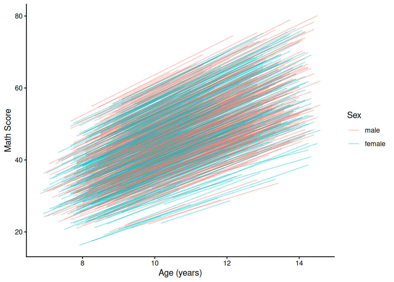
ggplot(
  data = mydata,
  mapping = aes(
    x = ageYears,
    y = math,
    group = id)) +
  geom_line() +
  labs(
    x = "Age (years)",
    y = "Math Score"
  ) +
  theme_classic()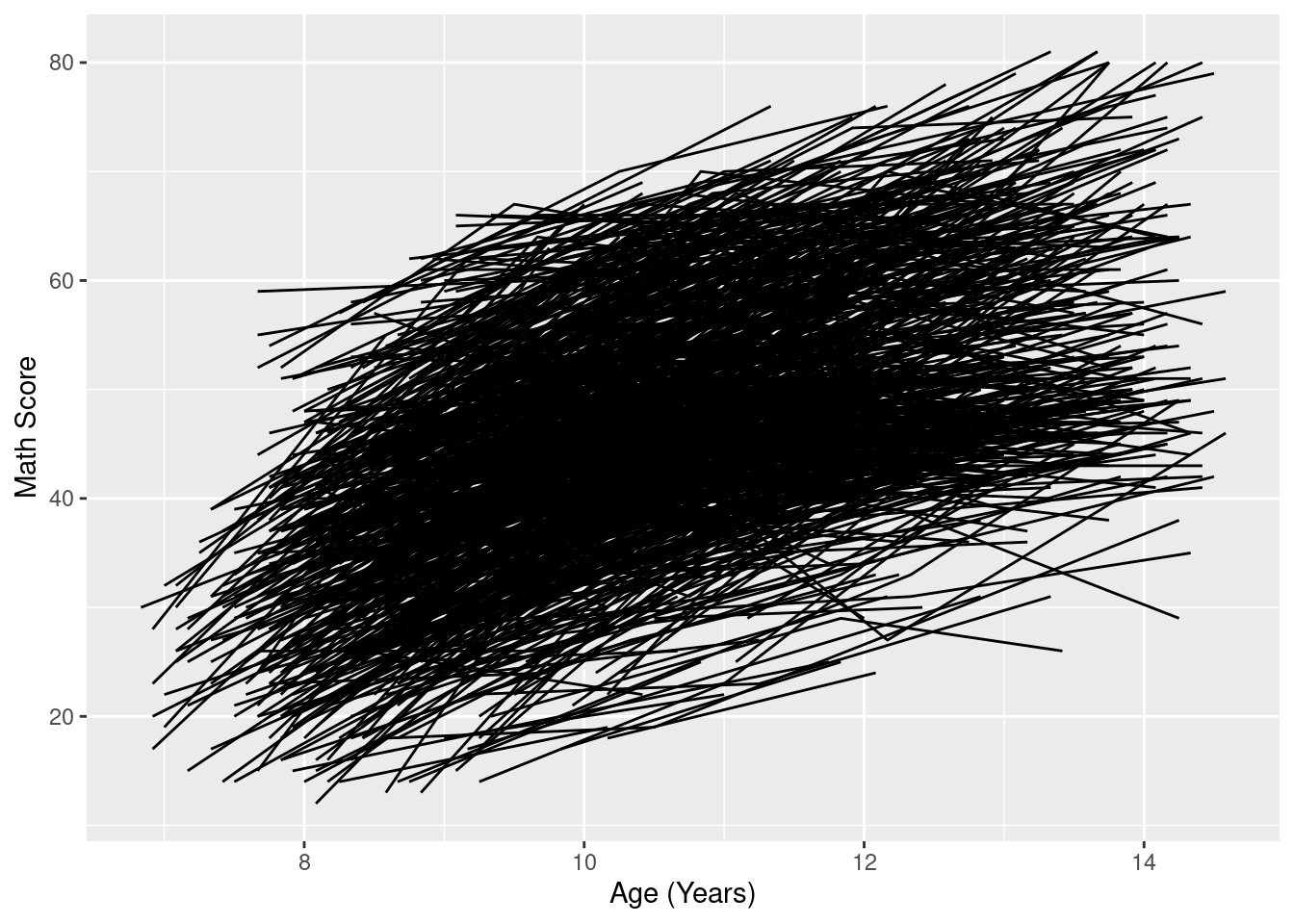

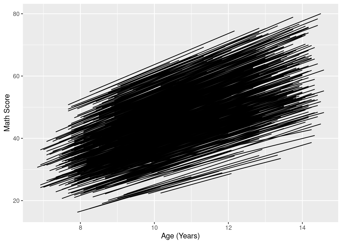
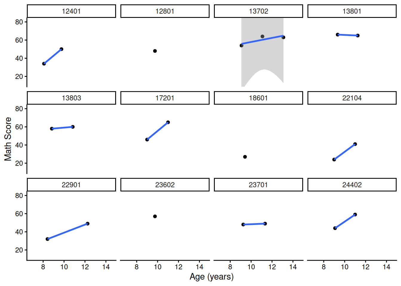
6.2 Faceted Plot

facetedPlots <- mydata |>
  ggplot(
    aes(
      x = ageYears,
      y = math,
      group = id
    )
  ) +
  geom_point() +
  geom_smooth(
    method = "lm"
  ) +
  coord_cartesian(
    ylim = c(min(mydata$math, na.rm = TRUE), max(mydata$math, na.rm = TRUE))) +
  labs(
    x = "Age (years)",
    y = "Math Score"
  ) +
  theme_classic() +
  ggforce::facet_wrap_paginate(
    ~ id,
    ncol = 4,
    nrow = 3)

num_pages <- ggforce::n_pages(facetedPlots)

for(i in 1:num_pages){
  print(facetedPlots + 
    ggforce::facet_wrap_paginate(
      ~ id,
      ncol = 4,
      nrow = 3,
      page = i))
}

7 Linear Mixed Models

The following models are models that are fit in a linear mixed modeling framework.

7.1 Growth Curve Models

7.1.1 Linear Growth Curve Model

7.1.1.1 lme4

linearMixedModel <- lmer(
  math ~ sex + ageYearsCentered + sex:ageYearsCentered + (1 + ageYearsCentered | id), # random intercepts and slopes; sex as a fixed-effect predictor of the intercepts and slopes
  data = mydata,
  REML = FALSE, #for ML
  na.action = na.exclude,
  control = lmerControl(optimizer = "bobyqa"))

summary(linearMixedModel)

Linear mixed model fit by maximum likelihood . t-tests use Satterthwaite's
  method [lmerModLmerTest]
Formula: 
math ~ sex + ageYearsCentered + sex:ageYearsCentered + (1 + ageYearsCentered |  
    id)
   Data: mydata
Control: lmerControl(optimizer = "bobyqa")

      AIC       BIC    logLik -2*log(L)  df.resid 
  15857.9   15903.5   -7920.9   15841.9      2213 

Scaled residuals: 
    Min      1Q  Median      3Q     Max 
-3.3750 -0.5174  0.0051  0.5239  2.6396 

Random effects:
 Groups   Name             Variance Std.Dev. Corr 
 id       (Intercept)      62.5365  7.9080        
          ageYearsCentered  0.6767  0.8226   0.08 
 Residual                  32.1505  5.6701        
Number of obs: 2221, groups:  id, 932

Fixed effects:
                            Estimate Std. Error        df t value Pr(>|t|)    
(Intercept)                 30.51401    0.56142 752.48747  54.352   <2e-16 ***
sexfemale                   -0.61290    0.79482 736.39886  -0.771    0.441    
ageYearsCentered             4.26792    0.11253 610.09410  37.925   <2e-16 ***
sexfemale:ageYearsCentered  -0.02558    0.16092 598.89155  -0.159    0.874    
---
Signif. codes:  0 '***' 0.001 '**' 0.01 '*' 0.05 '.' 0.1 ' ' 1

Correlation of Fixed Effects:
            (Intr) sexfml agYrsC
sexfemale   -0.706              
ageYrsCntrd -0.635  0.448       
sxfml:gYrsC  0.444 -0.631 -0.699

print(effectsize::standardize_parameters(
  linearMixedModel,
  method = "refit"),
  digits = 2)

# Standardization method: refit

Parameter                       | Std. Coef. |        95% CI
------------------------------------------------------------
(Intercept)                     |       0.03 | [-0.04, 0.10]
sex [female]                    |      -0.06 | [-0.15, 0.04]
ageYearsCentered                |       0.61 | [ 0.58, 0.64]
sex [female] × ageYearsCentered |  -3.67e-03 | [-0.05, 0.04]

performance::model_performance(linearMixedModel)

performance::r2(linearMixedModel)

# R2 for Mixed Models

  Conditional R2: 0.813
     Marginal R2: 0.358

7.1.1.1.1 Prototypical Growth Curve

newData <- expand.grid(
  female = c(0, 1),
  ageYears = c(
    min(mydata$ageYears, na.rm = TRUE),
    max(mydata$ageYears, na.rm = TRUE))
)

newData$ageYearsCentered <- newData$ageYears - min(newData$ageYears)

newData$sex <- NA
newData$sex[which(newData$female == 0)] <- "male"
newData$sex[which(newData$female == 1)] <- "female"
newData$sex <- as.factor(newData$sex)

newData$predictedValue <- predict( # predict.merMod
  linearMixedModel,
  newdata = newData,
  re.form = NA
)

ggplot(
  data = newData,
  mapping = aes(
    x = ageYears,
    y = predictedValue,
    color = sex)) +
  geom_line() +
  labs(
    x = "Age (years)",
    y = "Math Score",
    color = "Sex"
  ) +
  theme_classic()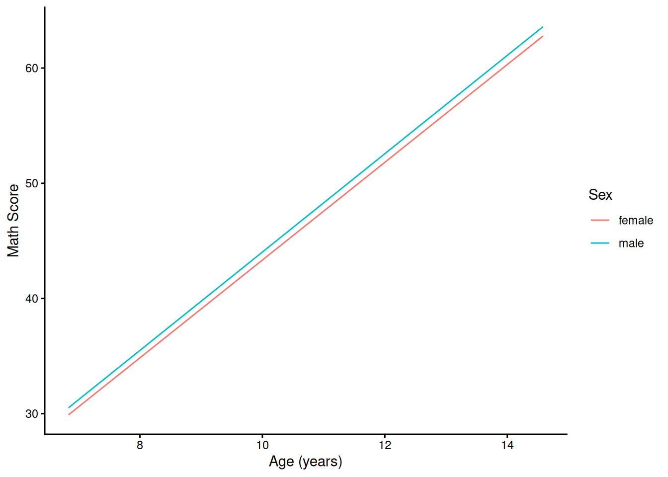

7.1.1.1.2 Individuals’ Growth Curves

mydata$predictedValue <- predict(
  linearMixedModel,
  newdata = mydata,
  re.form = NULL
)

ggplot(
  data = mydata,
  mapping = aes(
    x = ageYears,
    y = predictedValue,
    group = id,
    color = sex)) +
  geom_line(
    alpha = 0.4
  ) +
  labs(
    x = "Age (years)",
    y = "Math Score",
    color = "Sex"
  ) +
  theme_classic()

7.1.1.1.3 Individuals’ Trajectories Overlaid with Prototypical Trajectory

ggplot(
  data = mydata,
  mapping = aes(
    x = ageYears,
    y = predictedValue,
    group = id)) +
  geom_line( # individuals' trajectories
    color = "gray",
    alpha = 0.5
  ) +
  geom_line( # prototypical trajectory
    data = newData,
    mapping = aes(
      x = ageYears,
      y = predictedValue,
      group = sex,
      color = sex),
    linewidth = 2) +
  labs(
    x = "Age (years)",
    y = "Math Score",
    color = "Sex"
  ) +
  theme_classic()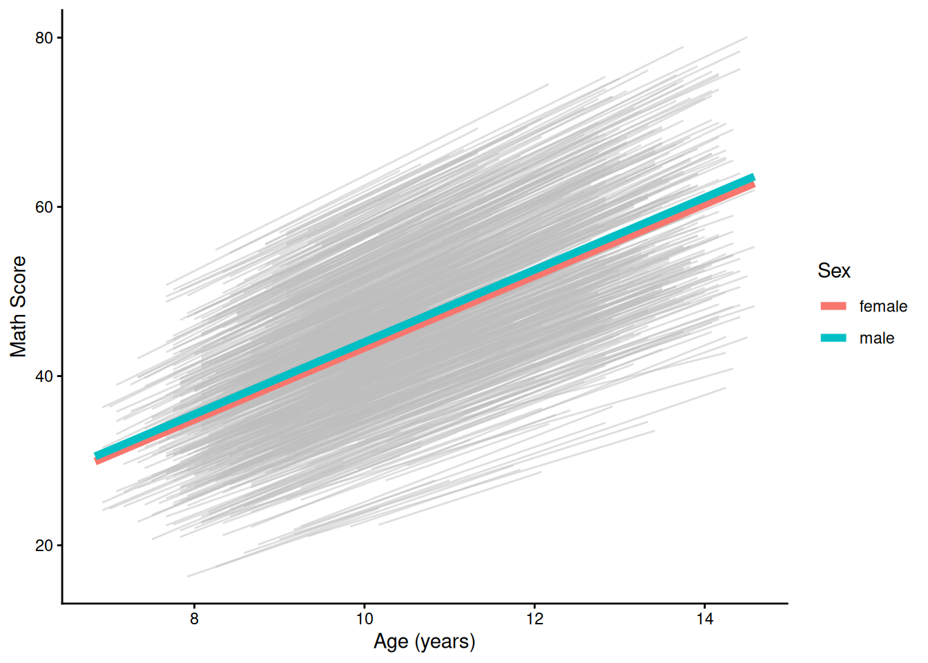

7.1.1.1.4 Extract Random Effects

ranef(linearMixedModel)

$id
     (Intercept) ageYearsCentered
201     1.125314        0.2140257
303   -12.515509       -0.6614897
2702   12.257492        0.4307630
4303    2.727958        0.2850021
5002    1.943701        0.1707896
5005    4.045983        0.1202867

with conditional variances for "id" 

7.1.1.1.5 Extract Participant-Specific Coefficients

coef(linearMixedModel)

$id
     (Intercept)  sexfemale ageYearsCentered sexfemale:ageYearsCentered
201     31.63933 -0.6128956         4.481949                -0.02558493
303     17.99850 -0.6128956         3.606434                -0.02558493
2702    42.77150 -0.6128956         4.698686                -0.02558493
4303    33.24197 -0.6128956         4.552925                -0.02558493
5002    32.45771 -0.6128956         4.438713                -0.02558493
5005    34.55999 -0.6128956         4.388210                -0.02558493

attr(,"class")
[1] "coef.mer"

7.1.1.2 nlme

linearMixedModel_nlme <- lme(
  math ~ sex + ageYearsCentered + sex:ageYearsCentered, # sex as a fixed-effect predictor of the intercepts and slopes
  random = ~ 1 + ageYearsCentered|id, # random intercepts and slopes
  data = mydata,
  method = "ML",
  na.action = na.exclude)

summary(linearMixedModel_nlme)

Linear mixed-effects model fit by maximum likelihood
  Data: mydata 
       AIC     BIC    logLik
  15857.85 15903.5 -7920.926

Random effects:
 Formula: ~1 + ageYearsCentered | id
 Structure: General positive-definite, Log-Cholesky parametrization
                 StdDev    Corr  
(Intercept)      7.9079987 (Intr)
ageYearsCentered 0.8225933 0.082 
Residual         5.6701380       

Fixed effects:  math ~ sex + ageYearsCentered + sex:ageYearsCentered 
                               Value Std.Error   DF  t-value p-value
(Intercept)                30.514011 0.5619217 1287 54.30296  0.0000
sexfemale                  -0.612896 0.7955333  930 -0.77042  0.4412
ageYearsCentered            4.267923 0.1126360 1287 37.89130  0.0000
sexfemale:ageYearsCentered -0.025585 0.1610671 1287 -0.15885  0.8738
 Correlation: 
                           (Intr) sexfml agYrsC
sexfemale                  -0.706              
ageYearsCentered           -0.635  0.448       
sexfemale:ageYearsCentered  0.444 -0.631 -0.699

Standardized Within-Group Residuals:
         Min           Q1          Med           Q3          Max 
-3.375034869 -0.517409797  0.005105047  0.523910718  2.639557775 

Number of Observations: 2221
Number of Groups: 932 

print(effectsize::standardize_parameters(
  linearMixedModel_nlme,
  method = "refit"),
  digits = 2)

# Standardization method: refit

Parameter                       | Std. Coef. |        95% CI
------------------------------------------------------------
(Intercept)                     |       0.03 | [-0.04, 0.10]
sex [female]                    |      -0.06 | [-0.15, 0.04]
ageYearsCentered                |       0.61 | [ 0.58, 0.64]
sex [female] × ageYearsCentered |  -3.67e-03 | [-0.05, 0.04]

performance::model_performance(linearMixedModel_nlme)

performance::r2(linearMixedModel_nlme)

# R2 for Mixed Models

  Conditional R2: 0.813
     Marginal R2: 0.358

7.1.1.3 R-Squared

The marginal \(R^2\) is the proportion of variance in the outcome variable that is accounted for by the fixed effects in the model, whereas the conditional \(R^2\) is the proportion of variance in the outcome variable that is accounted for by the fixed and random effects in the model.

performance::r2(linearMixedModel)

# R2 for Mixed Models

  Conditional R2: 0.813
     Marginal R2: 0.358

performance::r2(linearMixedModel_nlme)

# R2 for Mixed Models

  Conditional R2: 0.813
     Marginal R2: 0.358

7.1.1.4 Intraclass Correlation Coefficent

icc(linearMixedModel)

icc(linearMixedModel_nlme)

7.1.2 Growth Curve Model with Timepoint-Specific Errors

Adapted from Usami & Murayama (2018):

timepointSpecificErrorsMixedModel <- lmer(
  math ~ sex + ageYearsCentered + sex:ageYearsCentered + (1 | id) + (1 | ageYearsCentered), # timepoint-specific errors: observations are cross-classified with person and timepoint; sex as a fixed-effect predictor of the intercepts and slopes
  data = mydata,
  REML = FALSE, #for ML
  na.action = na.exclude,
  control = lmerControl(optimizer = "bobyqa"))

summary(timepointSpecificErrorsMixedModel)

Linear mixed model fit by maximum likelihood . t-tests use Satterthwaite's
  method [lmerModLmerTest]
Formula: math ~ sex + ageYearsCentered + sex:ageYearsCentered + (1 | id) +  
    (1 | ageYearsCentered)
   Data: mydata
Control: lmerControl(optimizer = "bobyqa")

      AIC       BIC    logLik -2*log(L)  df.resid 
  15808.6   15848.5   -7897.3   15794.6      2214 

Scaled residuals: 
    Min      1Q  Median      3Q     Max 
-3.5409 -0.5191  0.0051  0.5093  2.7345 

Random effects:
 Groups           Name        Variance Std.Dev.
 id               (Intercept) 76.219   8.730   
 ageYearsCentered (Intercept)  4.503   2.122   
 Residual                     30.842   5.554   
Number of obs: 2221, groups:  id, 932; ageYearsCentered, 94

Fixed effects:
                             Estimate Std. Error         df t value Pr(>|t|)
(Intercept)                  29.87438    0.75758  211.81838  39.434   <2e-16
sexfemale                    -0.38123    0.82243 1960.43213  -0.464    0.643
ageYearsCentered              4.26419    0.14813  132.95739  28.786   <2e-16
sexfemale:ageYearsCentered   -0.08143    0.14596 1364.56012  -0.558    0.577
                              
(Intercept)                ***
sexfemale                     
ageYearsCentered           ***
sexfemale:ageYearsCentered    
---
Signif. codes:  0 '***' 0.001 '**' 0.01 '*' 0.05 '.' 0.1 ' ' 1

Correlation of Fixed Effects:
            (Intr) sexfml agYrsC
sexfemale   -0.545              
ageYrsCntrd -0.758  0.321       
sxfml:gYrsC  0.356 -0.652 -0.482

print(effectsize::standardize_parameters(
  timepointSpecificErrorsMixedModel,
  method = "refit"),
  digits = 2)

# Standardization method: refit

Parameter                       | Std. Coef. |         95% CI
-------------------------------------------------------------
(Intercept)                     |      -1.27 | [-1.39, -1.15]
sex [female]                    |      -0.03 | [-0.16,  0.10]
ageYearsCentered                |       0.33 | [ 0.31,  0.36]
sex [female] × ageYearsCentered |  -6.36e-03 | [-0.03,  0.02]

performance::model_performance(timepointSpecificErrorsMixedModel)

performance::r2(timepointSpecificErrorsMixedModel)

# R2 for Mixed Models

  Conditional R2: 0.821
     Marginal R2: 0.352

7.1.3 Quadratic Growth Curve Model

When using higher-order polynomials, we could specify contrast codes for time to reduce multicollinearity between the linear and quadratic growth factors: https://tdjorgensen.github.io/SEM-in-Ed-compendium/ch27.html#saturated-growth-model (archived at https://perma.cc/88YL-USLC)

factorLoadings <- poly(
  x = c(0,1,2,3), # times (can allow unequal spacing)
  degree = 2)

factorLoadings

              1    2
[1,] -0.6708204  0.5
[2,] -0.2236068 -0.5
[3,]  0.2236068 -0.5
[4,]  0.6708204  0.5
attr(,"coefs")
attr(,"coefs")$alpha
[1] 1.5 1.5

attr(,"coefs")$norm2
[1] 1 4 5 4

attr(,"degree")
[1] 1 2
attr(,"class")
[1] "poly"   "matrix"

linearLoadings <- factorLoadings[,1]
quadraticLoadings <- factorLoadings[,2]

linearLoadings

[1] -0.6708204 -0.2236068  0.2236068  0.6708204

quadraticLoadings

[1]  0.5 -0.5 -0.5  0.5

7.1.3.1 Fit Model

quadraticGCM <- lmer(
  math ~ sex + ageYearsCentered + ageYearsCenteredSquared + sex:ageYearsCentered + sex:ageYearsCenteredSquared + (1 + ageYearsCentered | id), # random intercepts and linear slopes; fixed quadratic slopes; sex as a fixed-effect predictor of the intercepts and slopes
  data = mydata,
  REML = FALSE, #for ML
  na.action = na.exclude,
  control = lmerControl(optimizer = "bobyqa"))

summary(quadraticGCM)

Linear mixed model fit by maximum likelihood . t-tests use Satterthwaite's
  method [lmerModLmerTest]
Formula: 
math ~ sex + ageYearsCentered + ageYearsCenteredSquared + sex:ageYearsCentered +  
    sex:ageYearsCenteredSquared + (1 + ageYearsCentered | id)
   Data: mydata
Control: lmerControl(optimizer = "bobyqa")

      AIC       BIC    logLik -2*log(L)  df.resid 
  15666.9   15724.0   -7823.5   15646.9      2211 

Scaled residuals: 
    Min      1Q  Median      3Q     Max 
-3.3660 -0.4945  0.0048  0.5085  2.4377 

Random effects:
 Groups   Name             Variance Std.Dev. Corr  
 id       (Intercept)      69.8860  8.3598         
          ageYearsCentered  0.7099  0.8426   -0.05 
 Residual                  27.1959  5.2150         
Number of obs: 2221, groups:  id, 932

Fixed effects:
                                    Estimate Std. Error         df t value
(Intercept)                         23.43112    0.84914 1380.85816  27.594
sexfemale                            0.61167    1.18734 1370.91791   0.515
ageYearsCentered                     8.79334    0.42555 1381.21301  20.664
ageYearsCenteredSquared             -0.57623    0.05255 1382.10819 -10.966
sexfemale:ageYearsCentered          -0.62379    0.60301 1386.34429  -1.034
sexfemale:ageYearsCenteredSquared    0.05700    0.07582 1393.17373   0.752
                                  Pr(>|t|)    
(Intercept)                         <2e-16 ***
sexfemale                            0.607    
ageYearsCentered                    <2e-16 ***
ageYearsCenteredSquared             <2e-16 ***
sexfemale:ageYearsCentered           0.301    
sexfemale:ageYearsCenteredSquared    0.452    
---
Signif. codes:  0 '***' 0.001 '**' 0.01 '*' 0.05 '.' 0.1 ' ' 1

Correlation of Fixed Effects:
            (Intr) sexfml agYrsC agYrCS sxf:YC
sexfemale   -0.715                            
ageYrsCntrd -0.836  0.598                     
agYrsCntrdS  0.759 -0.543 -0.969              
sxfml:gYrsC  0.590 -0.829 -0.706  0.683       
sxfml:gYrCS -0.526  0.751  0.671 -0.693 -0.968

print(effectsize::standardize_parameters(
  quadraticGCM,
  method = "refit"),
  digits = 2)

# Standardization method: refit

Parameter                              | Std. Coef. |         95% CI
--------------------------------------------------------------------
(Intercept)                            |       0.02 | [-0.05,  0.08]
sex [female]                           |      -0.06 | [-0.15,  0.04]
ageYearsCentered                       |       1.26 | [ 1.14,  1.38]
ageYearsCenteredSquared                |      -0.67 | [-0.79, -0.55]
sex [female] × ageYearsCentered        |      -0.09 | [-0.26,  0.08]
sex [female] × ageYearsCenteredSquared |       0.07 | [-0.11,  0.24]

performance::model_performance(quadraticGCM)

performance::r2(quadraticGCM)

# R2 for Mixed Models

  Conditional R2: 0.840
     Marginal R2: 0.372

This is equivalent to:

quadraticGCM <- lmer(
  math ~ sex + ageYearsCentered + I(ageYearsCentered^2) + sex:ageYearsCentered + sex:I(ageYearsCentered^2) + (1 + ageYearsCentered | id), # random intercepts and slopes; sex as a fixed-effect predictor of the intercepts and slopes
  data = mydata,
  REML = FALSE, #for ML
  na.action = na.exclude,
  control = lmerControl(optimizer = "bobyqa"))

summary(quadraticGCM)

Linear mixed model fit by maximum likelihood . t-tests use Satterthwaite's
  method [lmerModLmerTest]
Formula: 
math ~ sex + ageYearsCentered + I(ageYearsCentered^2) + sex:ageYearsCentered +  
    sex:I(ageYearsCentered^2) + (1 + ageYearsCentered | id)
   Data: mydata
Control: lmerControl(optimizer = "bobyqa")

      AIC       BIC    logLik -2*log(L)  df.resid 
  15666.9   15724.0   -7823.5   15646.9      2211 

Scaled residuals: 
    Min      1Q  Median      3Q     Max 
-3.3660 -0.4945  0.0048  0.5085  2.4377 

Random effects:
 Groups   Name             Variance Std.Dev. Corr  
 id       (Intercept)      69.8860  8.3598         
          ageYearsCentered  0.7099  0.8426   -0.05 
 Residual                  27.1959  5.2150         
Number of obs: 2221, groups:  id, 932

Fixed effects:
                                  Estimate Std. Error         df t value
(Intercept)                       23.43112    0.84914 1380.85816  27.594
sexfemale                          0.61167    1.18734 1370.91791   0.515
ageYearsCentered                   8.79334    0.42555 1381.21301  20.664
I(ageYearsCentered^2)             -0.57623    0.05255 1382.10819 -10.966
sexfemale:ageYearsCentered        -0.62379    0.60301 1386.34429  -1.034
sexfemale:I(ageYearsCentered^2)    0.05700    0.07582 1393.17373   0.752
                                Pr(>|t|)    
(Intercept)                       <2e-16 ***
sexfemale                          0.607    
ageYearsCentered                  <2e-16 ***
I(ageYearsCentered^2)             <2e-16 ***
sexfemale:ageYearsCentered         0.301    
sexfemale:I(ageYearsCentered^2)    0.452    
---
Signif. codes:  0 '***' 0.001 '**' 0.01 '*' 0.05 '.' 0.1 ' ' 1

Correlation of Fixed Effects:
            (Intr) sexfml agYrsC I(YC^2 sxf:YC
sexfemale   -0.715                            
ageYrsCntrd -0.836  0.598                     
I(gYrsCn^2)  0.759 -0.543 -0.969              
sxfml:gYrsC  0.590 -0.829 -0.706  0.683       
sxf:I(YC^2) -0.526  0.751  0.671 -0.693 -0.968

print(effectsize::standardize_parameters(
  quadraticGCM,
  method = "refit"),
  digits = 2)

# Standardization method: refit

Parameter                         | Std. Coef. |         95% CI
---------------------------------------------------------------
(Intercept)                       |       0.17 | [ 0.10,  0.24]
sex [female]                      |      -0.07 | [-0.17,  0.03]
ageYearsCentered                  |       0.64 | [ 0.61,  0.67]
ageYearsCentered^2                |      -0.15 | [-0.18, -0.12]
sex [female] × ageYearsCentered   |      -0.03 | [-0.07,  0.01]
sex [female] × ageYearsCentered^2 |       0.02 | [-0.02,  0.05]

performance::model_performance(quadraticGCM)

performance::r2(quadraticGCM)

# R2 for Mixed Models

  Conditional R2: 0.840
     Marginal R2: 0.372

7.1.3.2 Prototypical Growth Curve

newData <- expand.grid(
  female = c(0, 1),
  ageYears = seq(from = min(mydata$ageYears, na.rm = TRUE), to = max(mydata$ageYears, na.rm = TRUE), length.out = 10000))

newData$ageYearsCentered <- newData$ageYears - min(newData$ageYears)
newData$ageYearsCenteredSquared <- newData$ageYearsCentered ^ 2

newData$sex <- NA
newData$sex[which(newData$female == 0)] <- "male"
newData$sex[which(newData$female == 1)] <- "female"
newData$sex <- as.factor(newData$sex)

newData$predictedValue <- predict( # predict.merMod
  quadraticGCM,
  newdata = newData,
  re.form = NA
)

ggplot(
  data = newData,
  mapping = aes(
    x = ageYears,
    y = predictedValue,
    color = sex)) +
  geom_line() +
  labs(
    x = "Age (years)",
    y = "Math Score",
    color = "Sex"
  ) +
  theme_classic()

7.1.3.3 Individuals’ Growth Curves

mydata$predictedValue <- predict(
  quadraticGCM,
  newdata = mydata,
  re.form = NULL
)

ggplot(
  data = mydata,
  mapping = aes(
    x = ageYears,
    y = predictedValue,
    group = id,
    color = sex)) +
  geom_line(
    stat = "smooth",
    method = "lm",
    formula = y ~ x + I(x^2),
    se = FALSE,
    linewidth = 0.5,
    alpha = 0.4
  ) +
  labs(
    x = "Age (years)",
    y = "Math Score",
    color = "Sex"
  ) +
  theme_classic()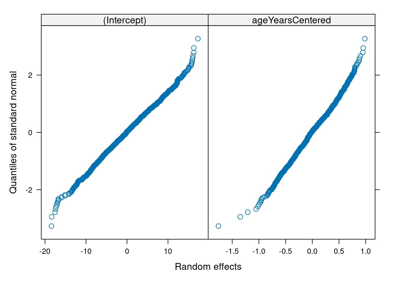

7.1.3.4 Individuals’ Trajectories Overlaid with Prototypical Trajectory

ggplot(
  data = mydata,
  mapping = aes(
    x = ageYears,
    y = predictedValue,
    group = id)) +
  geom_line( # individuals' trajectories
    stat = "smooth",
    method = "lm",
    formula = y ~ x + I(x^2),
    se = FALSE,
    linewidth = 0.5,
    color = "gray",
    alpha = 0.4
  ) +
  geom_line( # prototypical trajectory
    data = newData,
    mapping = aes(
      x = ageYears,
      y = predictedValue,
      group = sex,
      color = sex),
    linewidth = 2) +
  labs(
    x = "Age (years)",
    y = "Math Score",
    color = "Sex"
  ) +
  theme_classic()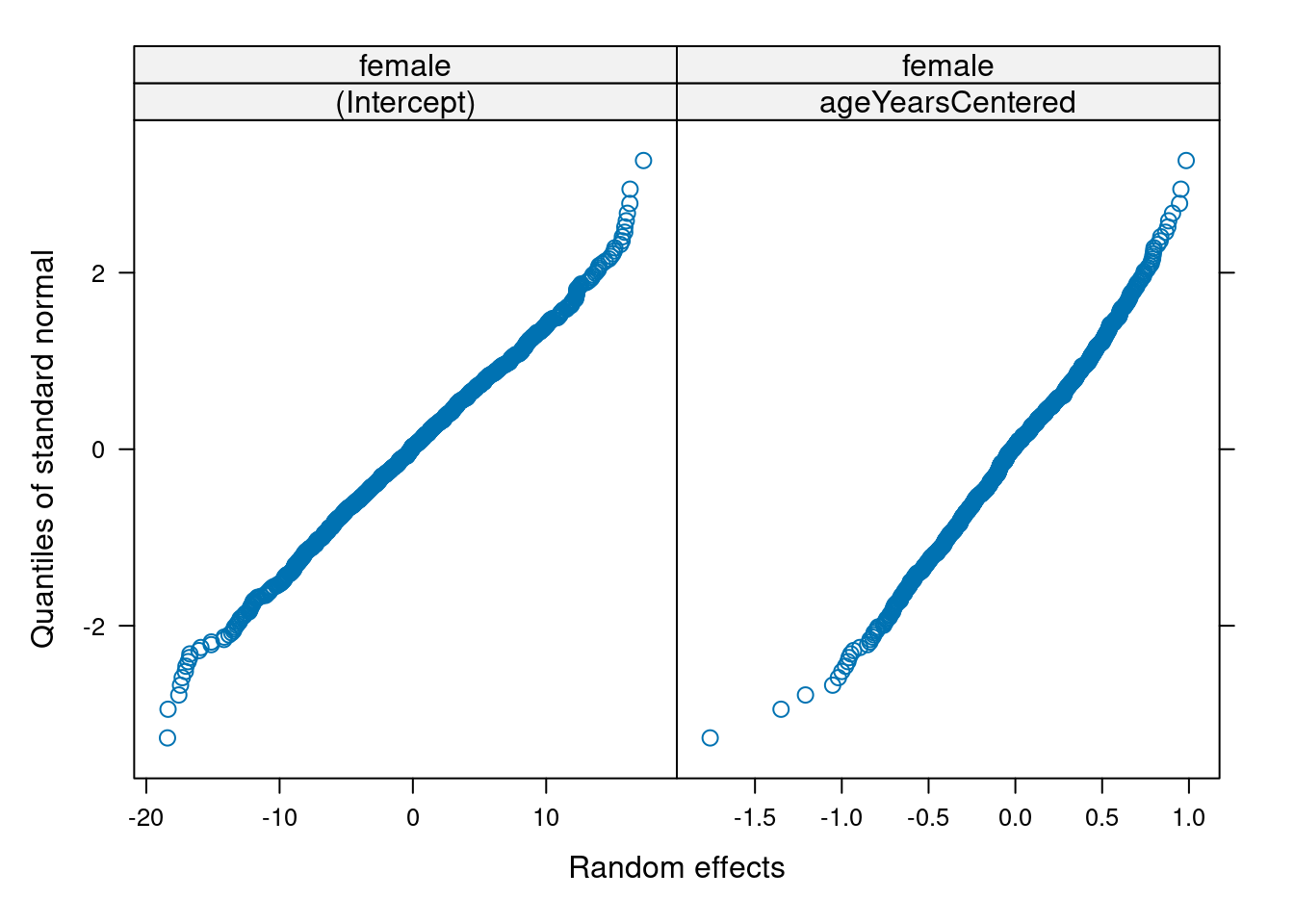

7.1.3.5 Extract Random Effects

ranef(quadraticGCM)

$id
     (Intercept) ageYearsCentered
201    0.3392871        0.2048916
303  -14.2395541       -0.5404362
2702  13.6789236        0.6053891
4303   1.8792650        0.2622509
5002   1.6186752        0.3766872
5005   5.0034217        0.1103062

with conditional variances for "id" 

7.1.4 Logarithmic Growth Curve Model

“an exponential pattern of change—in which change appears to ‘level off’ over time—can be approximated through linear (and potentially quadratic) slopes for a natural-log-transformed” version of time (Hoffman, 2025).

7.1.4.1 Fit Model

logGCM <- lmer(
  math ~ sex + log(ageYearsCentered + 1) + sex:log(ageYearsCentered + 1) + (1 + log(ageYearsCentered + 1) | id), # random intercepts and logarithmic slopes; sex as a fixed-effect predictor of the intercepts and slopes
  data = mydata,
  REML = FALSE, #for ML
  na.action = na.exclude,
  control = lmerControl(optimizer = "bobyqa"))

summary(logGCM)

Linear mixed model fit by maximum likelihood . t-tests use Satterthwaite's
  method [lmerModLmerTest]
Formula: math ~ sex + log(ageYearsCentered + 1) + sex:log(ageYearsCentered +  
    1) + (1 + log(ageYearsCentered + 1) | id)
   Data: mydata
Control: lmerControl(optimizer = "bobyqa")

      AIC       BIC    logLik -2*log(L)  df.resid 
  15656.4   15702.0   -7820.2   15640.4      2213 

Scaled residuals: 
    Min      1Q  Median      3Q     Max 
-3.4781 -0.5109  0.0083  0.5166  2.3670 

Random effects:
 Groups   Name                      Variance Std.Dev. Corr  
 id       (Intercept)               73.30    8.562          
          log(ageYearsCentered + 1) 12.23    3.497    -0.25 
 Residual                           27.09    5.205          
Number of obs: 2221, groups:  id, 932

Fixed effects:
                                    Estimate Std. Error       df t value
(Intercept)                          18.3941     0.7558 561.5187  24.336
sexfemale                             0.5112     1.0625 527.7083   0.481
log(ageYearsCentered + 1)            18.9931     0.4537 567.3593  41.862
sexfemale:log(ageYearsCentered + 1)  -0.8417     0.6405 525.5385  -1.314
                                    Pr(>|t|)    
(Intercept)                           <2e-16 ***
sexfemale                              0.631    
log(ageYearsCentered + 1)             <2e-16 ***
sexfemale:log(ageYearsCentered + 1)    0.189    
---
Signif. codes:  0 '***' 0.001 '**' 0.01 '*' 0.05 '.' 0.1 ' ' 1

Correlation of Fixed Effects:
            (Intr) sexfml l(YC+1
sexfemale   -0.711              
lg(gYrsC+1) -0.818  0.582       
sxfm:(YC+1)  0.580 -0.813 -0.708

print(effectsize::standardize_parameters(
  logGCM,
  method = "refit"),
  digits = 2)

# Standardization method: refit

Parameter                                 | Std. Coef. |         95% CI
-----------------------------------------------------------------------
(Intercept)                               |      -3.34 | [-3.51, -3.18]
sex [female]                              |       0.04 | [-0.19,  0.28]
ageYearsCentered + 1 [log]                |       2.47 | [ 2.35,  2.59]
sex [female] × ageYearsCentered + 1 [log] |      -0.07 | [-0.24,  0.10]

performance::model_performance(logGCM)

performance::r2(logGCM)

# R2 for Mixed Models

  Conditional R2: 0.842
     Marginal R2: 0.376

7.1.4.2 Prototypical Growth Curve

newData <- expand.grid(
  female = c(0, 1),
  ageYears = seq(from = min(mydata$ageYears, na.rm = TRUE), to = max(mydata$ageYears, na.rm = TRUE), length.out = 10000))

newData$ageYearsCentered <- newData$ageYears - min(newData$ageYears)

newData$sex <- NA
newData$sex[which(newData$female == 0)] <- "male"
newData$sex[which(newData$female == 1)] <- "female"
newData$sex <- as.factor(newData$sex)

newData$predictedValue <- predict( # predict.merMod
  logGCM,
  newdata = newData,
  re.form = NA
)

ggplot(
  data = newData,
  mapping = aes(
    x = ageYears,
    y = predictedValue,
    color = sex)) +
  geom_line() +
  labs(
    x = "Age (years)",
    y = "Math Score",
    color = "Sex"
  ) +
  theme_classic()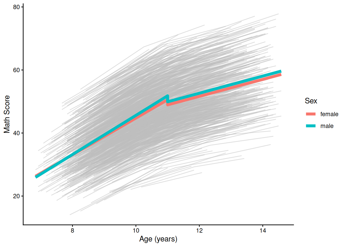

7.1.4.3 Individuals’ Growth Curves

mydata$predictedValue <- predict(
  logGCM,
  newdata = mydata,
  re.form = NULL
)

ggplot(
  data = mydata,
  mapping = aes(
    x = ageYears,
    y = predictedValue,
    group = id,
    color = sex)) +
  geom_line(
    stat = "smooth",
    method = "lm",
    formula = y ~ log(x + 1),
    se = FALSE,
    linewidth = 0.5,
    alpha = 0.4
  ) +
  labs(
    x = "Age (years)",
    y = "Math Score",
    color = "Sex"
  ) +
  theme_classic()

7.1.4.4 Individuals’ Trajectories Overlaid with Prototypical Trajectory

ggplot(
  data = mydata,
  mapping = aes(
    x = ageYears,
    y = predictedValue,
    group = id)) +
  geom_line( # individuals' trajectories
    stat = "smooth",
    method = "lm",
    formula = y ~ log(x + 1),
    se = FALSE,
    linewidth = 0.5,
    color = "gray",
    alpha = 0.4
  ) +
  geom_line( # prototypical trajectory
    data = newData,
    mapping = aes(
      x = ageYears,
      y = predictedValue,
      group = sex,
      color = sex),
    linewidth = 2) +
  labs(
    x = "Age (years)",
    y = "Math Score",
    color = "Sex"
  ) +
  theme_classic()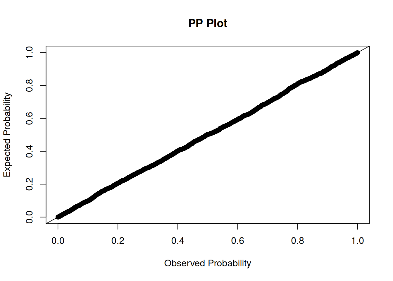

7.1.4.5 Extract Random Effects

ranef(logGCM)

$id
     (Intercept) log(ageYearsCentered + 1)
201   -0.2588159                 0.8989296
303  -12.3975047                -2.4573699
2702  12.6440791                 1.8110490
4303   1.2022598                 1.1227735
5002   1.1987292                 1.1430279
5005   4.5589766                 0.6030853

with conditional variances for "id" 

7.1.5 Spline Growth Curve Model

7.1.5.1 Create Knot

mydata$knot <- NA
mydata$knot[which(mydata$ageYears <= 11)] <- 0
mydata$knot[which(mydata$ageYears > 11)] <- 1

7.1.5.2 Fit Model

splineGCM <- lmer(
  math ~ sex + ageYearsCentered + sex:ageYearsCentered + knot + knot:ageYearsCentered + sex:knot + sex:knot:ageYearsCentered + (1 + ageYearsCentered | id), # random intercepts and linear slopes; fixed quadratic slopes; sex as a fixed-effect predictor of the intercepts and slopes
  data = mydata,
  REML = FALSE, #for ML
  na.action = na.exclude,
  control = lmerControl(optimizer = "bobyqa"))

summary(splineGCM)

Linear mixed model fit by maximum likelihood . t-tests use Satterthwaite's
  method [lmerModLmerTest]
Formula: math ~ sex + ageYearsCentered + sex:ageYearsCentered + knot +  
    knot:ageYearsCentered + sex:knot + sex:knot:ageYearsCentered +  
    (1 + ageYearsCentered | id)
   Data: mydata
Control: lmerControl(optimizer = "bobyqa")

      AIC       BIC    logLik -2*log(L)  df.resid 
  15691.2   15759.6   -7833.6   15667.2      2209 

Scaled residuals: 
    Min      1Q  Median      3Q     Max 
-3.3041 -0.5021 -0.0075  0.5034  2.4850 

Random effects:
 Groups   Name             Variance Std.Dev. Corr  
 id       (Intercept)      68.3568  8.2678         
          ageYearsCentered  0.7018  0.8377   -0.03 
 Residual                  27.7772  5.2704         
Number of obs: 2221, groups:  id, 932

Fixed effects:
                                 Estimate Std. Error        df t value Pr(>|t|)
(Intercept)                       25.9318     0.7222 1223.0139  35.909  < 2e-16
sexfemale                          0.3473     1.0060 1208.6807   0.345    0.730
ageYearsCentered                   6.2092     0.2328 1374.3269  26.674  < 2e-16
knot                              12.6515     1.8238 1241.0685   6.937 6.43e-12
sexfemale:ageYearsCentered        -0.3785     0.3240 1373.1043  -1.168    0.243
ageYearsCentered:knot             -3.4908     0.3746 1283.6771  -9.318  < 2e-16
sexfemale:knot                    -1.2105     2.6098 1234.2550  -0.464    0.643
sexfemale:ageYearsCentered:knot    0.3530     0.5383 1279.7386   0.656    0.512
                                   
(Intercept)                     ***
sexfemale                          
ageYearsCentered                ***
knot                            ***
sexfemale:ageYearsCentered         
ageYearsCentered:knot           ***
sexfemale:knot                     
sexfemale:ageYearsCentered:knot    
---
Signif. codes:  0 '***' 0.001 '**' 0.01 '*' 0.05 '.' 0.1 ' ' 1

Correlation of Fixed Effects:
            (Intr) sexfml agYrsC knot   sxf:YC agYrC: sxfml:
sexfemale   -0.718                                          
ageYrsCntrd -0.786  0.564                                   
knot        -0.267  0.192  0.266                            
sxfml:gYrsC  0.565 -0.776 -0.718 -0.191                     
agYrsCntrd:  0.470 -0.337 -0.568 -0.925  0.408              
sexfeml:knt  0.187 -0.259 -0.186 -0.699  0.262  0.646       
sxfml:gYrC: -0.327  0.455  0.395  0.644 -0.559 -0.696 -0.927

print(effectsize::standardize_parameters(
  splineGCM,
  method = "refit"),
  digits = 2)

# Standardization method: refit

Parameter                                | Std. Coef. |         95% CI
----------------------------------------------------------------------
(Intercept)                              |       0.23 | [ 0.15,  0.30]
sex [female]                             |      -0.08 | [-0.19,  0.03]
ageYearsCentered                         |       0.69 | [ 0.63,  0.74]
knot                                     |      -0.02 | [-0.07,  0.04]
sex [female] × ageYearsCentered          |      -0.03 | [-0.11,  0.04]
ageYearsCentered × knot                  |      -0.25 | [-0.30, -0.19]
sex [female] × knot                      |   4.24e-03 | [-0.08,  0.08]
(sex [female] × ageYearsCentered) × knot |       0.02 | [-0.05,  0.10]

performance::model_performance(splineGCM)

performance::r2(splineGCM)

# R2 for Mixed Models

  Conditional R2: 0.836
     Marginal R2: 0.370

7.1.5.3 Prototypical Growth Curve

newData <- expand.grid(
  female = c(0, 1),
  ageYears = seq(from = min(mydata$ageYears, na.rm = TRUE), to = max(mydata$ageYears, na.rm = TRUE), length.out = 10000))

newData$ageYearsCentered <- newData$ageYears - min(newData$ageYears)

newData$knot <- NA
newData$knot[which(newData$ageYears <= 11)] <- 0
newData$knot[which(newData$ageYears > 11)] <- 1

newData$sex <- NA
newData$sex[which(newData$female == 0)] <- "male"
newData$sex[which(newData$female == 1)] <- "female"
newData$sex <- as.factor(newData$sex)

newData$predictedValue <- predict( # predict.merMod
  splineGCM,
  newdata = newData,
  re.form = NA
)

ggplot(
  data = newData,
  mapping = aes(
    x = ageYears,
    y = predictedValue,
    color = sex)) +
  geom_line() +
  labs(
    x = "Age (years)",
    y = "Math Score",
    color = "Sex"
  ) +
  theme_classic()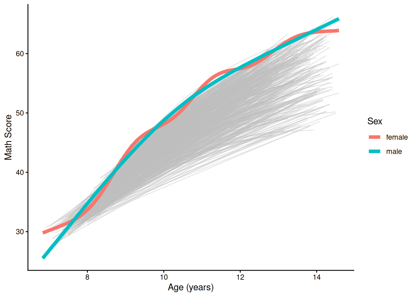

7.1.5.4 Individuals’ Growth Curves

mydata$predictedValue <- predict(
  splineGCM,
  newdata = mydata,
  re.form = NULL
)

ggplot(
  data = mydata,
  mapping = aes(
    x = ageYears,
    y = predictedValue,
    group = id,
    color = sex)) +
  geom_line(
    alpha = 0.4
  ) +
  labs(
    x = "Age (years)",
    y = "Math Score",
    color = "Sex"
  ) +
  theme_classic()

7.1.5.5 Individuals’ Trajectories Overlaid with Prototypical Trajectory

ggplot(
  data = mydata,
  mapping = aes(
    x = ageYears,
    y = predictedValue,
    group = id)) +
  geom_line( # individuals' trajectories
    color = "gray",
    alpha = 0.5
  ) +
  geom_line( # prototypical trajectory
    data = newData,
    mapping = aes(
      x = ageYears,
      y = predictedValue,
      group = sex,
      color = sex),
    linewidth = 2) +
  labs(
    x = "Age (years)",
    y = "Math Score",
    color = "Sex"
  ) +
  theme_classic()

7.1.5.6 Extract Random Effects

ranef(splineGCM)

$id
     (Intercept) ageYearsCentered
201     0.652145        0.2083235
303   -13.900383       -0.5384101
2702   13.248702        0.4885446
4303    2.123618        0.2695865
5002    1.813505        0.3311535
5005    4.914571        0.1306295

with conditional variances for "id" 

7.1.6 Accelerated Longitudinal Study: Accounting for Age at T1 and Time in Study

Per Hoffman (here, archived at https://perma.cc/6X8R-EX44; and here, archived at https://perma.cc/25JY-JE8P), use age at baseline (i.e., T1; or birth year) instead of mean age to lessen bias from attrition‐related missing data.

7.1.6.1 Linear

acceleratedLongitudinalMixedModel_linear <- lmer(
  math ~ timeInStudy*sex*ageAtT1Centered + (1 + timeInStudy | id),
  data = mydata,
  REML = FALSE, #for ML
  na.action = na.exclude,
  control = lmerControl(optimizer = "bobyqa"))

summary(acceleratedLongitudinalMixedModel_linear)

Linear mixed model fit by maximum likelihood . t-tests use Satterthwaite's
  method [lmerModLmerTest]
Formula: math ~ timeInStudy * sex * ageAtT1Centered + (1 + timeInStudy |  
    id)
   Data: mydata
Control: lmerControl(optimizer = "bobyqa")

      AIC       BIC    logLik -2*log(L)  df.resid 
  15825.5   15893.9   -7900.7   15801.5      2209 

Scaled residuals: 
    Min      1Q  Median      3Q     Max 
-3.3506 -0.5034  0.0041  0.5148  2.5209 

Random effects:
 Groups   Name        Variance Std.Dev. Corr 
 id       (Intercept) 71.3489  8.4468        
          timeInStudy  0.7547  0.8687   0.13 
 Residual             30.5886  5.5307        
Number of obs: 2221, groups:  id, 932

Fixed effects:
                                      Estimate Std. Error       df t value
(Intercept)                            30.4960     1.0769 923.7136  28.318
timeInStudy                             5.6213     0.2681 515.9405  20.968
sexfemale                              -0.5900     1.5106 925.1091  -0.391
ageAtT1Centered                         4.2875     0.4563 941.2874   9.397
timeInStudy:sexfemale                  -0.5706     0.3718 495.6079  -1.535
timeInStudy:ageAtT1Centered            -0.7289     0.1337 801.8462  -5.452
sexfemale:ageAtT1Centered              -0.0300     0.6566 942.8209  -0.046
timeInStudy:sexfemale:ageAtT1Centered   0.2496     0.1929 792.8030   1.294
                                      Pr(>|t|)    
(Intercept)                            < 2e-16 ***
timeInStudy                            < 2e-16 ***
sexfemale                                0.696    
ageAtT1Centered                        < 2e-16 ***
timeInStudy:sexfemale                    0.126    
timeInStudy:ageAtT1Centered           6.64e-08 ***
sexfemale:ageAtT1Centered                0.964    
timeInStudy:sexfemale:ageAtT1Centered    0.196    
---
Signif. codes:  0 '***' 0.001 '**' 0.01 '*' 0.05 '.' 0.1 ' ' 1

Correlation of Fixed Effects:
            (Intr) tmInSt sexfml agAT1C tmInS: tIS:AT s:AT1C
timeInStudy -0.264                                          
sexfemale   -0.713  0.188                                   
agAtT1Cntrd -0.906  0.260  0.646                            
tmInStdy:sx  0.191 -0.721 -0.261 -0.187                     
tmInSt:AT1C  0.216 -0.906 -0.154 -0.267  0.653              
sxfml:gAT1C  0.630 -0.181 -0.903 -0.695  0.256  0.185       
tmInS::AT1C -0.150  0.628  0.209  0.185 -0.899 -0.693 -0.261

print(effectsize::standardize_parameters(
  acceleratedLongitudinalMixedModel_linear,
  method = "refit"),
  digits = 2)

# Standardization method: refit

Parameter                                      | Std. Coef. |         95% CI
----------------------------------------------------------------------------
(Intercept)                                    |       0.02 | [-0.05,  0.08]
timeInStudy                                    |       0.58 | [ 0.55,  0.62]
sex [female]                                   |      -0.06 | [-0.16,  0.04]
ageAtT1Centered                                |       0.22 | [ 0.15,  0.28]
timeInStudy × sex [female]                     |      -0.01 | [-0.06,  0.04]
timeInStudy × ageAtT1Centered                  |      -0.10 | [-0.13, -0.06]
sex [female] × ageAtT1Centered                 |       0.03 | [-0.06,  0.12]
(timeInStudy × sex [female]) × ageAtT1Centered |       0.03 | [-0.02,  0.08]

performance::model_performance(acceleratedLongitudinalMixedModel_linear)

performance::r2(acceleratedLongitudinalMixedModel_linear)

# R2 for Mixed Models

  Conditional R2: 0.821
     Marginal R2: 0.356

7.1.6.1.1 Prototypical Growth Curve

newData <- unique(mydata[,c("ageYears","ageAtT1","timeInStudy")])

newData$ageAtT1Centered <- newData$ageAtT1 - min(mydata$ageAtT1, na.rm = TRUE)

newData <- tidyr::expand_grid(
  newData,
  female = c(0, 1)
)

newData$sex <- NA
newData$sex[which(newData$female == 0)] <- "male"
newData$sex[which(newData$female == 1)] <- "female"
newData$sex <- as.factor(newData$sex)

newData$predictedValue <- predict( # predict.merMod
  acceleratedLongitudinalMixedModel_linear,
  newdata = newData,
  re.form = NA
)

ggplot(
  data = newData,
  mapping = aes(
    x = ageYears,
    y = predictedValue,
    color = sex)) +
  geom_smooth() + #for jagged line: geom_line()
  labs(
    x = "Age (years)",
    y = "Math Score",
    color = "Sex"
  ) +
  theme_classic()

7.1.6.1.2 Individuals’ Growth Curves

mydata$predictedValue <- predict(
  acceleratedLongitudinalMixedModel_linear,
  newdata = mydata,
  re.form = NULL
)

ggplot(
  data = mydata,
  mapping = aes(
    x = ageYears,
    y = predictedValue,
    group = id,
    color = sex)) +
  geom_line(
    alpha = 0.4
  ) +
  labs(
    x = "Age (years)",
    y = "Math Score",
    color = "Sex"
  ) +
  theme_classic()

7.1.6.1.3 Individuals’ Trajectories Overlaid with Prototypical Trajectory

ggplot(
  data = mydata,
  mapping = aes(
    x = ageYears,
    y = predictedValue,
    group = id)) +
  geom_line( # individuals' trajectories
    color = "gray",
    alpha = 0.5
  ) +
  geom_smooth( # prototypical trajectory
    data = newData,
    mapping = aes(
      x = ageYears,
      y = predictedValue,
      group = sex,
      color = sex),
    linewidth = 2) +
  labs(
    x = "Age (years)",
    y = "Math Score",
    color = "Sex"
  ) +
  theme_classic()

7.1.6.2 Quadratic

acceleratedLongitudinalMixedModel_quadratic <- lmer(
  math ~ timeInStudy*sex*ageAtT1Centered + timeInStudySquared*sex*ageAtT1Centered + ageAtT1CenteredSquared + (1 + timeInStudy | id),
  data = mydata,
  REML = FALSE, #for ML
  na.action = na.exclude,
  control = lmerControl(optimizer = "bobyqa"))

summary(acceleratedLongitudinalMixedModel_quadratic)

Linear mixed model fit by maximum likelihood . t-tests use Satterthwaite's
  method [lmerModLmerTest]
Formula: math ~ timeInStudy * sex * ageAtT1Centered + timeInStudySquared *  
    sex * ageAtT1Centered + ageAtT1CenteredSquared + (1 + timeInStudy |  
    id)
   Data: mydata
Control: lmerControl(optimizer = "bobyqa")

      AIC       BIC    logLik -2*log(L)  df.resid 
  15652.6   15749.6   -7809.3   15618.6      2204 

Scaled residuals: 
    Min      1Q  Median      3Q     Max 
-3.2689 -0.5022 -0.0008  0.5033  2.2831 

Random effects:
 Groups   Name        Variance Std.Dev. Corr 
 id       (Intercept) 72.8962  8.5379        
          timeInStudy  0.8827  0.9395   0.03 
 Residual             26.1840  5.1170        
Number of obs: 2221, groups:  id, 932

Fixed effects:
                                               Estimate Std. Error         df
(Intercept)                                    24.70634    1.46211 1001.51224
timeInStudy                                    10.59805    0.62300 1111.53789
sexfemale                                      -0.08203    1.51844  989.54150
ageAtT1Centered                                 8.63457    1.06400 1002.81922
timeInStudySquared                             -0.97702    0.13105 1281.23846
ageAtT1CenteredSquared                         -0.75767    0.19273  998.93944
timeInStudy:sexfemale                          -1.98056    0.88286 1115.72074
timeInStudy:ageAtT1Centered                    -2.16322    0.30585 1089.28752
sexfemale:ageAtT1Centered                      -0.20420    0.65764  992.70315
sexfemale:timeInStudySquared                    0.34751    0.18308 1279.76216
ageAtT1Centered:timeInStudySquared              0.25089    0.07586 1285.46075
timeInStudy:sexfemale:ageAtT1Centered           0.89953    0.44344 1106.64698
sexfemale:ageAtT1Centered:timeInStudySquared   -0.18389    0.10878 1297.47442
                                             t value Pr(>|t|)    
(Intercept)                                   16.898  < 2e-16 ***
timeInStudy                                   17.011  < 2e-16 ***
sexfemale                                     -0.054 0.956927    
ageAtT1Centered                                8.115 1.41e-15 ***
timeInStudySquared                            -7.455 1.65e-13 ***
ageAtT1CenteredSquared                        -3.931 9.03e-05 ***
timeInStudy:sexfemale                         -2.243 0.025070 *  
timeInStudy:ageAtT1Centered                   -7.073 2.71e-12 ***
sexfemale:ageAtT1Centered                     -0.311 0.756239    
sexfemale:timeInStudySquared                   1.898 0.057900 .  
ageAtT1Centered:timeInStudySquared             3.307 0.000968 ***
timeInStudy:sexfemale:ageAtT1Centered          2.029 0.042746 *  
sexfemale:ageAtT1Centered:timeInStudySquared  -1.691 0.091164 .  
---
Signif. codes:  0 '***' 0.001 '**' 0.01 '*' 0.05 '.' 0.1 ' ' 1

print(effectsize::standardize_parameters(
  acceleratedLongitudinalMixedModel_quadratic,
  method = "refit"),
  digits = 2)

# Standardization method: refit

Parameter                                             | Std. Coef. |         95% CI
-----------------------------------------------------------------------------------
(Intercept)                                           |       0.01 | [-0.06,  0.08]
timeInStudy                                           |       0.88 | [ 0.80,  0.96]
sex [female]                                          |      -0.07 | [-0.17,  0.02]
ageAtT1Centered                                       |       0.47 | [ 0.32,  0.62]
timeInStudySquared                                    |      -0.34 | [-0.43, -0.24]
ageAtT1CenteredSquared                                |      -0.27 | [-0.40, -0.13]
timeInStudy × sex [female]                            |      -0.03 | [-0.14,  0.09]
timeInStudy × ageAtT1Centered                         |      -0.28 | [-0.36, -0.20]
sex [female] × ageAtT1Centered                        |       0.02 | [-0.08,  0.11]
sex [female] × timeInStudySquared                     |      -0.01 | [-0.16,  0.13]
ageAtT1Centered × timeInStudySquared                  |       0.16 | [ 0.07,  0.26]
(timeInStudy × sex [female]) × ageAtT1Centered        |       0.12 | [ 0.00,  0.23]
(sex [female] × ageAtT1Centered) × timeInStudySquared |      -0.12 | [-0.26,  0.02]

performance::model_performance(acceleratedLongitudinalMixedModel_quadratic)

performance::r2(acceleratedLongitudinalMixedModel_quadratic)

# R2 for Mixed Models

  Conditional R2: 0.842
     Marginal R2: 0.364

7.1.6.2.1 Prototypical Growth Curve

newData <- unique(mydata[,c("ageYears","ageAtT1","timeInStudy")])

newData$ageAtT1Centered <- newData$ageAtT1 - min(mydata$ageAtT1, na.rm = TRUE)
newData$timeInStudySquared <- newData$timeInStudy ^ 2
newData$ageAtT1CenteredSquared <- newData$ageAtT1Centered ^2

newData <- tidyr::expand_grid(
  newData,
  female = c(0, 1)
)

newData$sex <- NA
newData$sex[which(newData$female == 0)] <- "male"
newData$sex[which(newData$female == 1)] <- "female"
newData$sex <- as.factor(newData$sex)

newData$predictedValue <- predict( # predict.merMod
  acceleratedLongitudinalMixedModel_quadratic,
  newdata = newData,
  re.form = NA
)

ggplot(
  data = newData,
  mapping = aes(
    x = ageYears,
    y = predictedValue,
    color = sex)) +
  geom_smooth() + #for jagged line: geom_line()
  labs(
    x = "Age (years)",
    y = "Math Score",
    color = "Sex"
  ) +
  theme_classic()

7.1.6.2.2 Individuals’ Growth Curves

mydata$predictedValue <- predict(
  acceleratedLongitudinalMixedModel_quadratic,
  newdata = mydata,
  re.form = NULL
)

ggplot(
  data = mydata,
  mapping = aes(
    x = ageYears,
    y = predictedValue,
    group = id,
    color = sex)) +
  geom_smooth(
    method = "lm",
    formula = y ~ x + I(x^2),
    se = FALSE,
    linewidth = 0.5,
    alpha = 0.4
  ) +
  labs(
    x = "Age (years)",
    y = "Math Score",
    color = "Sex"
  ) +
  theme_classic()

7.1.6.2.3 Individuals’ Trajectories Overlaid with Prototypical Trajectory

ggplot(
  data = mydata,
  mapping = aes(
    x = ageYears,
    y = predictedValue,
    group = id)) +
  geom_smooth( # individuals' trajectories
    method = "lm",
    formula = y ~ x + I(x^2),
    se = FALSE,
    linewidth = 0.4,
    color = "gray",
    alpha = 0.5
  ) +
  geom_smooth( # prototypical trajectory
    data = newData,
    mapping = aes(
      x = ageYears,
      y = predictedValue,
      group = sex,
      color = sex),
    linewidth = 2) +
  labs(
    x = "Age (years)",
    y = "Math Score",
    color = "Sex"
  ) +
  theme_classic()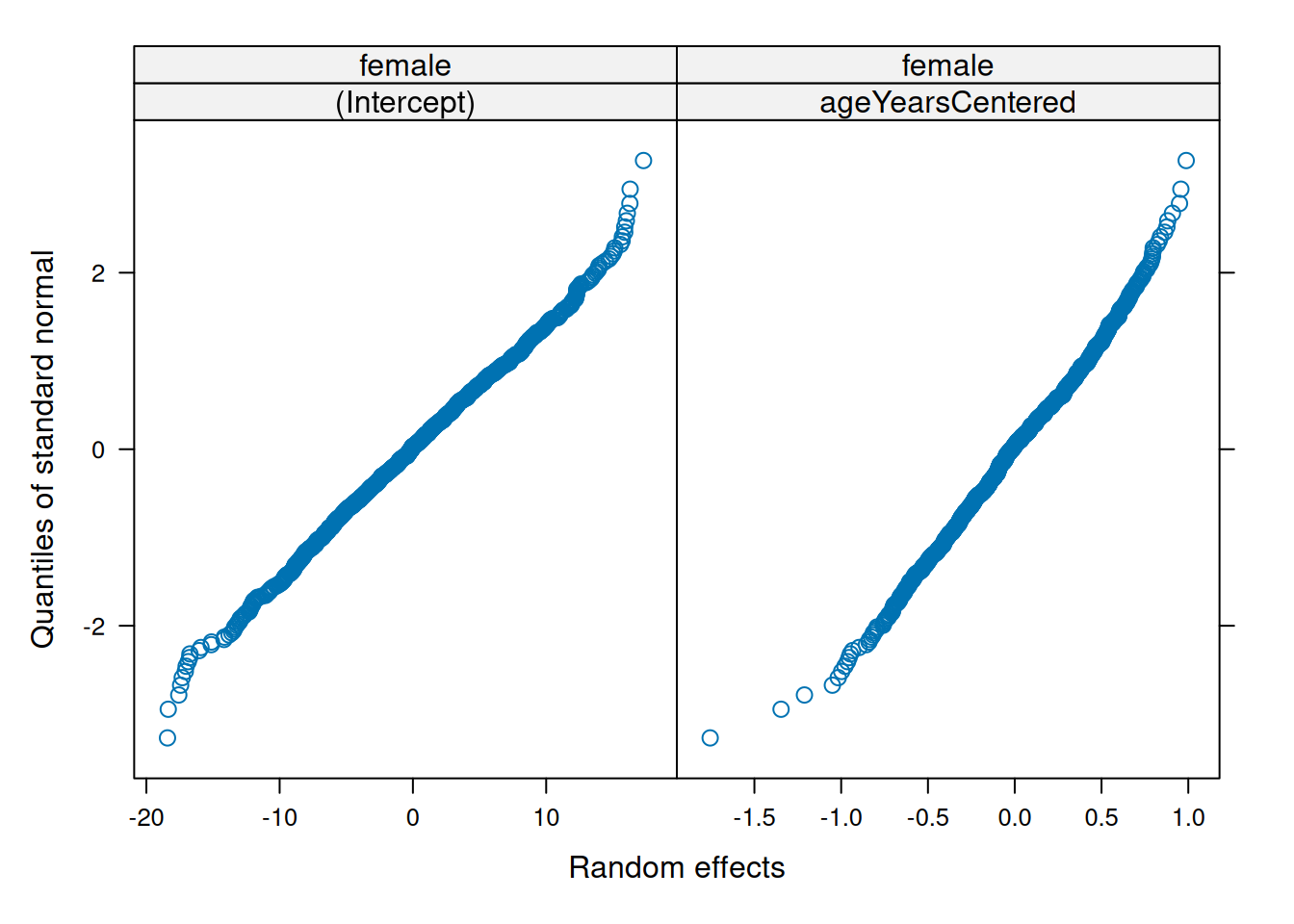

8 Generalized Linear Mixed Models

https://bbolker.github.io/mixedmodels-misc/glmmFAQ.html (archived at https://perma.cc/9RFS-BCE7; source code: https://github.com/bbolker/mixedmodels-misc/blob/master/glmmFAQ.rmd)

8.1 lmer

generalizedLinearMixedModel <- glmer(
  outcome ~ female + ageYearsCentered + (ageYearsCentered | id),
  family = poisson(link = "log"),
  data = mydata,
  na.action = na.exclude)

summary(generalizedLinearMixedModel)

Generalized linear mixed model fit by maximum likelihood (Laplace
  Approximation) [glmerMod]
 Family: poisson  ( log )
Formula: outcome ~ female + ageYearsCentered + (ageYearsCentered | id)
   Data: mydata

      AIC       BIC    logLik -2*log(L)  df.resid 
   9329.7    9363.9   -4658.8    9317.7      2215 

Scaled residuals: 
    Min      1Q  Median      3Q     Max 
-2.0331 -0.5546 -0.0205  0.5350  5.0222 

Random effects:
 Groups Name             Variance  Std.Dev. Corr  
 id     (Intercept)      0.0058309 0.07636        
        ageYearsCentered 0.0002845 0.01687  -1.00 
Number of obs: 2221, groups:  id, 932

Fixed effects:
                 Estimate Std. Error z value Pr(>|z|)    
(Intercept)      1.343986   0.026879  50.001   <2e-16 ***
female           0.007439   0.021268   0.350   0.7265    
ageYearsCentered 0.010279   0.005804   1.771   0.0766 .  
---
Signif. codes:  0 '***' 0.001 '**' 0.01 '*' 0.05 '.' 0.1 ' ' 1

Correlation of Fixed Effects:
            (Intr) female
female      -0.421       
ageYrsCntrd -0.831  0.036
optimizer (Nelder_Mead) convergence code: 0 (OK)
boundary (singular) fit: see help('isSingular')

print(effectsize::standardize_parameters(
  generalizedLinearMixedModel,
  method = "refit"),
  digits = 2)

# Standardization method: refit

Parameter        | Std. Coef. |        95% CI
---------------------------------------------
(Intercept)      |       1.39 | [ 1.37, 1.41]
female           |   3.72e-03 | [-0.02, 0.02]
ageYearsCentered |       0.02 | [ 0.00, 0.04]

- Response is unstandardized.

performance::model_performance(generalizedLinearMixedModel)

performance::r2(generalizedLinearMixedModel)

[1] NA

8.2 MASS

glmmPQLmodel <- glmmPQL(
  outcome ~ female + ageYearsCentered,
  random = ~ 1 + ageYearsCentered|id,
  family = poisson(link = "log"),
  data = mydata)

summary(glmmPQLmodel)

Linear mixed-effects model fit by maximum likelihood
  Data: mydata 
  AIC BIC logLik
   NA  NA     NA

Random effects:
 Formula: ~1 + ageYearsCentered | id
 Structure: General positive-definite, Log-Cholesky parametrization
                 StdDev       Corr  
(Intercept)      5.533290e-05 (Intr)
ageYearsCentered 9.320922e-08 0     
Residual         1.014184e+00       

Variance function:
 Structure: fixed weights
 Formula: ~invwt 
Fixed effects:  outcome ~ female + ageYearsCentered 
                     Value   Std.Error   DF  t-value p-value
(Intercept)      1.3453017 0.027100741 1288 49.64077  0.0000
female           0.0074130 0.021543030  930  0.34410  0.7308
ageYearsCentered 0.0100806 0.005850753 1288  1.72296  0.0851
 Correlation: 
                 (Intr) female
female           -0.423       
ageYearsCentered -0.829  0.036

Standardized Within-Group Residuals:
        Min          Q1         Med          Q3         Max 
-2.00970268 -0.55110605 -0.02158036  0.53179575  4.98914420 

Number of Observations: 2221
Number of Groups: 932 

print(effectsize::standardize_parameters(
  glmmPQLmodel,
  method = "refit"),
  digits = 2)

# Standardization method: refit

Parameter        | Std. Coef. |        95% CI
---------------------------------------------
(Intercept)      |       1.39 | [ 1.37, 1.41]
female           |   3.71e-03 | [-0.02, 0.02]
ageYearsCentered |       0.02 | [ 0.00, 0.04]

- Response is unstandardized.

8.3 MCMCglmm

MCMCglmmModel <- MCMCglmm(
  outcome ~ female + ageYearsCentered,
  random = ~ us(ageYearsCentered):id,
  family = "poisson",
  data = na.omit(mydata[,c("id","outcome","female","ageYearsCentered")]))

                       MCMC iteration = 0

 Acceptance ratio for liability set 1 = 0.000410

                       MCMC iteration = 1000

 Acceptance ratio for liability set 1 = 0.439819

                       MCMC iteration = 2000

 Acceptance ratio for liability set 1 = 0.439977

                       MCMC iteration = 3000

 Acceptance ratio for liability set 1 = 0.444608

                       MCMC iteration = 4000

 Acceptance ratio for liability set 1 = 0.496749

                       MCMC iteration = 5000

 Acceptance ratio for liability set 1 = 0.490778

                       MCMC iteration = 6000

 Acceptance ratio for liability set 1 = 0.512362

                       MCMC iteration = 7000

 Acceptance ratio for liability set 1 = 0.428231

                       MCMC iteration = 8000

 Acceptance ratio for liability set 1 = 0.412336

                       MCMC iteration = 9000

 Acceptance ratio for liability set 1 = 0.471726

                       MCMC iteration = 10000

 Acceptance ratio for liability set 1 = 0.428491

                       MCMC iteration = 11000

 Acceptance ratio for liability set 1 = 0.400078

                       MCMC iteration = 12000

 Acceptance ratio for liability set 1 = 0.346435

                       MCMC iteration = 13000

 Acceptance ratio for liability set 1 = 0.276170

summary(MCMCglmmModel)

 Iterations = 3001:12991
 Thinning interval  = 10
 Sample size  = 1000 

 DIC: 9323.524 

 G-structure:  ~us(ageYearsCentered):id

                                     post.mean  l-95% CI  u-95% CI eff.samp
ageYearsCentered:ageYearsCentered.id 6.754e-06 1.087e-08 4.053e-05    7.788

 R-structure:  ~units

      post.mean l-95% CI u-95% CI eff.samp
units   0.00877 0.001634  0.01728    7.797

 Location effects: outcome ~ female + ageYearsCentered 

                 post.mean  l-95% CI  u-95% CI eff.samp  pMCMC    
(Intercept)       1.338707  1.281096  1.387614    55.58 <0.001 ***
female            0.007688 -0.031193  0.052271    58.65  0.706    
ageYearsCentered  0.010561  0.000813  0.021420    57.32  0.046 *  
---
Signif. codes:  0 '***' 0.001 '**' 0.01 '*' 0.05 '.' 0.1 ' ' 1

9 Nonlinear Mixed Models

9.1 Generalized Additive Mixed Model

9.1.1 Fit Model

num_cores <- parallelly::availableCores() - 1
num_true_cores <- parallelly::availableCores(logical = FALSE) - 1

gamModel <- mgcv::gam(
  math ~ s(ageYearsCentered, by = sex) + s(id, ageYearsCentered, bs = "re"),
  data = mydata,
  nthreads = num_cores
)

summary(gamModel)

Family: gaussian 
Link function: identity 

Formula:
math ~ s(ageYearsCentered, by = sex) + s(id, ageYearsCentered, 
    bs = "re")

Parametric coefficients:
            Estimate Std. Error t value Pr(>|t|)    
(Intercept)  49.9227     0.3718   134.3   <2e-16 ***
---
Signif. codes:  0 '***' 0.001 '**' 0.01 '*' 0.05 '.' 0.1 ' ' 1

Approximate significance of smooth terms:
                                 edf Ref.df     F p-value    
s(ageYearsCentered):sexmale   2.8831  3.613 219.7  <2e-16 ***
s(ageYearsCentered):sexfemale 6.2237  6.805 120.3  <2e-16 ***
s(id,ageYearsCentered)        0.9932  1.000 155.5  <2e-16 ***
---
Signif. codes:  0 '***' 0.001 '**' 0.01 '*' 0.05 '.' 0.1 ' ' 1

Rank: 18/20
R-sq.(adj) =  0.396   Deviance explained = 39.9%
GCV = 99.429  Scale est. = 98.933    n = 2221

print(effectsize::standardize_parameters(
  gamModel,
  method = "refit"),
  digits = 2)

# Standardization method: refit

Component    |                                  Parameter | Std. Coef. |        95% CI
--------------------------------------------------------------------------------------
conditional  |                                (Intercept) |  -1.80e-03 | [-0.04, 0.03]
smooth_terms |   Smooth term (ageYearsCentered) × sexmale |            |              
smooth_terms | Smooth term (ageYearsCentered) × sexfemale |            |              
smooth_terms |          Smooth term (id,ageYearsCentered) |            |              

performance::model_performance(gamModel)

performance::r2(gamModel)

$R2
Adjusted R2 
  0.3961561 

9.1.2 Prototypical Growth Curve

newData <- expand.grid(
  female = c(0, 1),
  ageYears = seq(from = min(mydata$ageYears, na.rm = TRUE), to = max(mydata$ageYears, na.rm = TRUE), length.out = 10000))

newData$ageYearsCentered <- newData$ageYears - min(newData$ageYears)
newData$ageYearsCenteredSquared <- newData$ageYearsCentered ^ 2

newData$sex <- NA
newData$sex[which(newData$female == 0)] <- "male"
newData$sex[which(newData$female == 1)] <- "female"
newData$sex <- as.factor(newData$sex)

# add a dummy id
newData$id <- mydata$id[1]

newData$predictedValue <- predict(
  gamModel,
  newdata = newData,
  exclude = "s(ageYearsCentered,id)"
)

ggplot(
  data = newData,
  mapping = aes(
    x = ageYears,
    y = predictedValue,
    color = sex)) +
  geom_line() +
  labs(
    x = "Age (years)",
    y = "Math Score",
    color = "Sex"
  ) +
  theme_classic()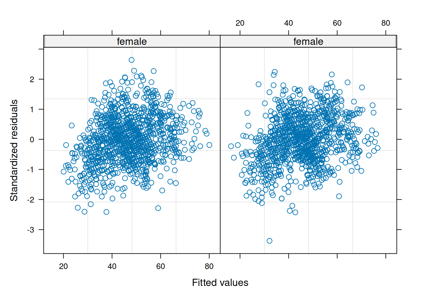

9.1.3 Individuals’ Growth Curves

mydata$predictedValue <- predict(
  gamModel,
  newdata = mydata
)

gamMethod <- function(formula, data, weights, ...) { # from here: https://stackoverflow.com/a/76762792/2029527 (archived at https://perma.cc/85C6-FKJ4)
  if(nrow(data) < 4) return(lm(y ~ x, data = data, ...))
  else  mgcv::gam(y ~ s(x, bs = "cs", k = 3), data = data, ...)
}

ggplot(
  data = mydata,
  mapping = aes(
    x = ageYears,
    y = predictedValue,
    group = id,
    color = sex)) +
  geom_line(
    stat = "smooth",
    method = gamMethod,
    se = FALSE,
    linewidth = 0.5,
    alpha = 0.4
  ) +
  labs(
    x = "Age (years)",
    y = "Math Score",
    color = "Sex"
  ) +
  theme_classic()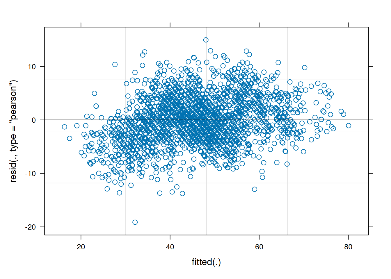

9.1.4 Individuals’ Trajectories Overlaid with Prototypical Trajectory

ggplot(
  data = mydata,
  mapping = aes(
    x = ageYears,
    y = predictedValue,
    group = id)) +
  geom_line( # individuals' trajectories
    stat = "smooth",
    method = gamMethod,
    se = FALSE,
    linewidth = 0.5,
    color = "gray",
    alpha = 0.4
  ) +
  geom_line( # prototypical trajectory
    data = newData,
    mapping = aes(
      x = ageYears,
      y = predictedValue,
      group = sex,
      color = sex),
    linewidth = 2) +
  labs(
    x = "Age (years)",
    y = "Math Score",
    color = "Sex"
  ) +
  theme_classic()

9.2 Asymptotic Growth

nonlinearModel <- nlme(
  height ~ SSasymp(age, Asym, R0, lrc),
  data = Loblolly,
  fixed = Asym + R0 + lrc ~ 1,
  random = Asym ~ 1)

summary(nonlinearModel)

Nonlinear mixed-effects model fit by maximum likelihood
  Model: height ~ SSasymp(age, Asym, R0, lrc) 
  Data: Loblolly 
      AIC      BIC   logLik
  239.486 251.6401 -114.743

Random effects:
 Formula: Asym ~ 1 | Seed
            Asym  Residual
StdDev: 3.650645 0.7188624

Fixed effects:  list(Asym ~ 1, R0 ~ 1, lrc ~ 1) 
         Value Std.Error DF   t-value p-value
Asym 101.44830 2.4616151 68  41.21209       0
R0    -8.62749 0.3179519 68 -27.13459       0
lrc   -3.23373 0.0342695 68 -94.36168       0
 Correlation: 
    Asym   R0    
R0   0.704       
lrc -0.908 -0.827

Standardized Within-Group Residuals:
        Min          Q1         Med          Q3         Max 
-2.23604174 -0.62389999  0.05912777  0.65724316  1.95790785 

Number of Observations: 84
Number of Groups: 14 

10 Disaggregation of Within-Person and Between-Person Effects

10.1 Pre-Model Computations

mydata_long$sexFactor <- factor(mydata_long$sex) # create a factor variable for sex

mydata_long$ageCentered <- mydata_long$age - min(mydata_long$age, na.rm = TRUE) # shift age so that intercepts represent the earliest age in the sample

mydata_long$ageCenteredSquared <- mydata_long$ageCentered ^ 2

mydata_long <- mydata_long |>
  group_by(ID) |>
  mutate(
    sleep_personMean = mean(sleep, na.rm = TRUE),
    sleep_personMeanCentered = sleep - sleep_personMean
  ) |>
  ungroup()

10.2 Fit the Model

In disaggregating within- and between-person effects, this model fits:

1. random intercepts and random linear slopes for subjects,
2. sex and sleep_personMean as time-invariant fixed-effect predictors of the intercepts and slopes, and
3. sleep_personMeanCentered as a time-varying fixed-effect predictor of depression.

withinBetweenPersonSleepModel_basic <- lmerTest::lmer(
  depression ~ sleep_personMean + sexFactor +              # time-invariant predictors of the intercepts
    sleep_personMeanCentered + ageCentered +               # time-varying predictors
    sleep_personMean:ageCentered + sexFactor:ageCentered + # time-invariant predictors of the slopes
    (1 + ageCentered | ID),
  data = mydata_long,
  na.action = na.exclude)

We can also extend the model to a quadratic model (or to any other functional form of change).

In disaggregating within- and between-person effects, this model fits:

1. random intercepts and random linear slopes and fixed quadratic slopes for subjects,
2. sex and sleep_personMean (and their interaction) as time-invariant fixed-effect predictors of the intercepts and slopes, and
3. sleep_personMeanCentered as a time-varying fixed-effect predictor of depression, with effects allowed to vary over age and by sex, including two‐ and three‐way interactions with age and sex.

The * symbol (unlike the : symbol) estimates all lower-order main effects and interactions, to simplify the syntax.

withinBetweenPersonSleepModel <- lmerTest::lmer(
  depression ~ sexFactor*sleep_personMean*ageCentered + 
    sexFactor*sleep_personMean*ageCenteredSquared + 
    sexFactor*sleep_personMeanCentered*ageCentered + 
    sexFactor*sleep_personMeanCentered*ageCenteredSquared + 
    (1 + ageCentered | ID), # model fails to converge with a random effect for ageCenteredSquared
  data = mydata_long,
  na.action = na.exclude)

10.3 Model Summary

summary(withinBetweenPersonSleepModel)

Linear mixed model fit by REML. t-tests use Satterthwaite's method [
lmerModLmerTest]
Formula: depression ~ sexFactor * sleep_personMean * ageCentered + sexFactor *  
    sleep_personMean * ageCenteredSquared + sexFactor * sleep_personMeanCentered *  
    ageCentered + sexFactor * sleep_personMeanCentered * ageCenteredSquared +  
    (1 + ageCentered | ID)
   Data: mydata_long

REML criterion at convergence: 4626.7

Scaled residuals: 
    Min      1Q  Median      3Q     Max 
-2.5691 -0.4181 -0.0233  0.3799  3.1684 

Random effects:
 Groups   Name        Variance Std.Dev. Corr 
 ID       (Intercept) 14.331   3.786         
          ageCentered  2.404   1.551    0.53 
 Residual              2.237   1.496         
Number of obs: 931, groups:  ID, 250

Fixed effects:
                                                           Estimate Std. Error
(Intercept)                                                24.00570    2.85852
sexFactormale                                              -5.01340    4.32597
sleep_personMean                                           -1.60234    0.35245
ageCentered                                                 6.31714    2.04483
ageCenteredSquared                                         -0.70171    0.56569
sleep_personMeanCentered                                   -1.23490    0.31669
sexFactormale:sleep_personMean                              0.33208    0.53553
sexFactormale:ageCentered                                  -9.59764    3.11058
sleep_personMean:ageCentered                               -0.89401    0.25235
sexFactormale:ageCenteredSquared                            2.42488    0.86957
sleep_personMean:ageCenteredSquared                         0.16374    0.06980
sexFactormale:sleep_personMeanCentered                      0.03113    0.45428
ageCentered:sleep_personMeanCentered                        1.09341    0.55380
ageCenteredSquared:sleep_personMeanCentered                -0.39972    0.18201
sexFactormale:sleep_personMean:ageCentered                  0.99055    0.38523
sexFactormale:sleep_personMean:ageCenteredSquared          -0.30129    0.10778
sexFactormale:ageCentered:sleep_personMeanCentered         -0.47191    0.77720
sexFactormale:ageCenteredSquared:sleep_personMeanCentered   0.25192    0.25677
                                                                 df t value
(Intercept)                                               261.31526   8.398
sexFactormale                                             261.53048  -1.159
sleep_personMean                                          261.37873  -4.546
ageCentered                                               667.32798   3.089
ageCenteredSquared                                        447.12110  -1.240
sleep_personMeanCentered                                  616.86197  -3.899
sexFactormale:sleep_personMean                            261.42255   0.620
sexFactormale:ageCentered                                 668.34418  -3.085
sleep_personMean:ageCentered                              667.55202  -3.543
sexFactormale:ageCenteredSquared                          453.87104   2.789
sleep_personMean:ageCenteredSquared                       446.91031   2.346
sexFactormale:sleep_personMeanCentered                    619.99241   0.069
ageCentered:sleep_personMeanCentered                      625.42997   1.974
ageCenteredSquared:sleep_personMeanCentered               644.97219  -2.196
sexFactormale:sleep_personMean:ageCentered                668.20437   2.571
sexFactormale:sleep_personMean:ageCenteredSquared         453.82812  -2.796
sexFactormale:ageCentered:sleep_personMeanCentered        641.12293  -0.607
sexFactormale:ageCenteredSquared:sleep_personMeanCentered 657.31531   0.981
                                                          Pr(>|t|)    
(Intercept)                                               2.92e-15 ***
sexFactormale                                             0.247552    
sleep_personMean                                          8.36e-06 ***
ageCentered                                               0.002090 ** 
ageCenteredSquared                                        0.215463    
sleep_personMeanCentered                                  0.000107 ***
sexFactormale:sleep_personMean                            0.535731    
sexFactormale:ageCentered                                 0.002116 ** 
sleep_personMean:ageCentered                              0.000424 ***
sexFactormale:ageCenteredSquared                          0.005516 ** 
sleep_personMean:ageCenteredSquared                       0.019425 *  
sexFactormale:sleep_personMeanCentered                    0.945382    
ageCentered:sleep_personMeanCentered                      0.048780 *  
ageCenteredSquared:sleep_personMeanCentered               0.028436 *  
sexFactormale:sleep_personMean:ageCentered                0.010345 *  
sexFactormale:sleep_personMean:ageCenteredSquared         0.005402 ** 
sexFactormale:ageCentered:sleep_personMeanCentered        0.543940    
sexFactormale:ageCenteredSquared:sleep_personMeanCentered 0.326910    
---
Signif. codes:  0 '***' 0.001 '**' 0.01 '*' 0.05 '.' 0.1 ' ' 1

print(effectsize::standardize_parameters(
  withinBetweenPersonSleepModel,
  method = "refit"),
  digits = 2)

# Standardization method: refit

Parameter                                                          | Std. Coef. |         95% CI
------------------------------------------------------------------------------------------------
(Intercept)                                                        |       0.31 | [ 0.18,  0.45]
sexFactor [male]                                                   |      -0.71 | [-0.91, -0.51]
sleep personMean                                                   |      -0.34 | [-0.48, -0.21]
ageCentered                                                        |      -0.14 | [-0.23, -0.06]
ageCenteredSquared                                                 |       0.32 | [ 0.25,  0.39]
sleep personMeanCentered                                           |      -0.09 | [-0.11, -0.06]
sexFactor [male] × sleep personMean                                |       0.11 | [-0.09,  0.31]
sexFactor [male] × ageCentered                                     |      -0.28 | [-0.40, -0.16]
sleep personMean × ageCentered                                     |      -0.15 | [-0.23, -0.06]
sexFactor [male] × ageCenteredSquared                              |   3.62e-03 | [-0.10,  0.11]
sleep personMean × ageCenteredSquared                              |       0.08 | [ 0.01,  0.15]
sexFactor [male] × sleep personMeanCentered                        |       0.02 | [-0.02,  0.05]
ageCentered × sleep personMeanCentered                             |       0.11 | [ 0.00,  0.22]
ageCenteredSquared × sleep personMeanCentered                      |      -0.12 | [-0.23, -0.01]
(sexFactor [male] × sleep personMean) × ageCentered                |       0.16 | [ 0.04,  0.28]
(sexFactor [male] × sleep personMean) × ageCenteredSquared         |      -0.15 | [-0.26, -0.05]
(sexFactor [male] × ageCentered) × sleep personMeanCentered        |      -0.05 | [-0.20,  0.11]
(sexFactor [male] × ageCenteredSquared) × sleep personMeanCentered |       0.08 | [-0.08,  0.23]

performance::r2(withinBetweenPersonSleepModel)

# R2 for Mixed Models

  Conditional R2: 0.950
     Marginal R2: 0.246

10.4 Plots

10.4.1 Between-Person Effect of Sleep

newData <- expand.grid(
  sexFactor = c("female", "male"),
  age = seq(
    from = min(mydata_long$age, na.rm = TRUE),
    to = max(mydata_long$age, na.rm = TRUE),
    length.out = 10000
  ),
  sleepFactor = c("low sleep", "high sleep")
)

newData$ageCentered <- newData$age - min(newData$age)
newData$ageCenteredSquared <- newData$ageCentered ^ 2

newData$sleep_personMean <- NA
newData$sleep_personMean[which(newData$sleepFactor == "low sleep" & newData$sexFactor == "female")] <- mean(mydata_long$sleep_personMean[which(mydata_long$sexFactor == "female")], na.rm = TRUE) - sd(mydata_long$sleep_personMean[which(mydata_long$sexFactor == "female")], na.rm = TRUE)

newData$sleep_personMean[which(newData$sleepFactor == "low sleep" & newData$sexFactor == "male")] <- mean(mydata_long$sleep_personMean[which(mydata_long$sexFactor == "male")], na.rm = TRUE) - sd(mydata_long$sleep_personMean[which(mydata_long$sexFactor == "male")], na.rm = TRUE)

newData$sleep_personMean[which(newData$sleepFactor == "high sleep" & newData$sexFactor == "female")] <- mean(mydata_long$sleep_personMean[which(mydata_long$sexFactor == "female")], na.rm = TRUE) + sd(mydata_long$sleep_personMean[which(mydata_long$sexFactor == "female")], na.rm = TRUE)

newData$sleep_personMean[which(newData$sleepFactor == "high sleep" & newData$sexFactor == "male")] <- mean(mydata_long$sleep_personMean[which(mydata_long$sexFactor == "male")], na.rm = TRUE) + sd(mydata_long$sleep_personMean[which(mydata_long$sexFactor == "male")], na.rm = TRUE)

newData$sleep_personMeanCentered <- 0

newData$modelImpliedDepression <- predict( # predict.merMod
  withinBetweenPersonSleepModel,
  newdata = newData,
  re.form = NA # include no random effects
)

ggplot(
  data = newData,
  mapping = aes(
    x = age,
    y = modelImpliedDepression,
    color = sexFactor,
    linetype = sleepFactor)) +
  geom_line() +
  labs(
    x = "Age (years)",
    y = "Depression Symptoms",
    color = "Sex",
    linetype = "Sleep"
  ) +
  theme_classic()

Between-Person Association Between Sleep and Depression

10.4.2 Within-Person Effect of Sleep

newData <- expand.grid(
  sexFactor = c("female", "male"),
  age = seq(
    from = min(mydata_long$age, na.rm = TRUE),
    to = max(mydata_long$age, na.rm = TRUE),
    length.out = 10000
  ),
  sleepFactor = c("low sleep", "high sleep")
)

newData$ageCentered <- newData$age - min(newData$age)
newData$ageCenteredSquared <- newData$ageCentered ^ 2

newData$sleep_personMean <- mean(mydata_long$sleep_personMean, na.rm = TRUE)

newData$sleep_personMeanCentered <- NA
newData$sleep_personMeanCentered[which(newData$sleepFactor == "low sleep" & newData$sexFactor == "female")] <- mean(mydata_long$sleep_personMeanCentered[which(mydata_long$sexFactor == "female")], na.rm = TRUE) - sd(mydata_long$sleep_personMeanCentered[which(mydata_long$sexFactor == "female")], na.rm = TRUE)

newData$sleep_personMeanCentered[which(newData$sleepFactor == "low sleep" & newData$sexFactor == "male")] <- mean(mydata_long$sleep_personMeanCentered[which(mydata_long$sexFactor == "male")], na.rm = TRUE) - sd(mydata_long$sleep_personMeanCentered[which(mydata_long$sexFactor == "male")], na.rm = TRUE)

newData$sleep_personMeanCentered[which(newData$sleepFactor == "high sleep" & newData$sexFactor == "female")] <- mean(mydata_long$sleep_personMeanCentered[which(mydata_long$sexFactor == "female")], na.rm = TRUE) + sd(mydata_long$sleep_personMeanCentered[which(mydata_long$sexFactor == "female")], na.rm = TRUE)

newData$sleep_personMeanCentered[which(newData$sleepFactor == "high sleep" & newData$sexFactor == "male")] <- mean(mydata_long$sleep_personMeanCentered[which(mydata_long$sexFactor == "male")], na.rm = TRUE) + sd(mydata_long$sleep_personMeanCentered[which(mydata_long$sexFactor == "male")], na.rm = TRUE)

newData$modelImpliedDepression <- predict( # predict.merMod
  withinBetweenPersonSleepModel,
  newdata = newData,
  re.form = NA # include no random effects
)

ggplot(
  data = newData,
  mapping = aes(
    x = age,
    y = modelImpliedDepression,
    color = sexFactor,
    linetype = sleepFactor)) +
  geom_line() +
  labs(
    x = "Age (years)",
    y = "Depression Symptoms",
    color = "Sex",
    linetype = "Sleep"
  ) +
  theme_classic()

Within-Person Association Between Sleep and Depression

11 Moderated Multilevel Models

Simonsohn (2024)

moderatedMultilevelModel <- mgcv::gam(
  math ~
    s(timeInStudy) +
    s(ageAtT1Centered) +
    ti(timeInStudy, ageAtT1Centered) +
    s(id, bs = "re") +
    s(id, by = timeInStudy, bs = "re"),
  data = mydata
)

summary(moderatedMultilevelModel)

Family: gaussian 
Link function: identity 

Formula:
math ~ s(timeInStudy) + s(ageAtT1Centered) + ti(timeInStudy, 
    ageAtT1Centered) + s(id, bs = "re") + s(id, by = timeInStudy, 
    bs = "re")

Parametric coefficients:
            Estimate Std. Error t value Pr(>|t|)    
(Intercept)  50.3660     0.4074   123.6   <2e-16 ***
---
Signif. codes:  0 '***' 0.001 '**' 0.01 '*' 0.05 '.' 0.1 ' ' 1

Approximate significance of smooth terms:
                                   edf Ref.df       F p-value    
s(timeInStudy)                  6.0969  6.186 138.163  <2e-16 ***
s(ageAtT1Centered)              6.6576  7.311  25.027  <2e-16 ***
ti(timeInStudy,ageAtT1Centered) 2.5460  3.440  14.883  <2e-16 ***
s(id)                           0.9979  1.000 189.934  <2e-16 ***
s(id):timeInStudy               0.1149  1.000   0.084   0.425    
---
Signif. codes:  0 '***' 0.001 '**' 0.01 '*' 0.05 '.' 0.1 ' ' 1

Rank: 32/37
R-sq.(adj) =  0.411   Deviance explained = 41.5%
GCV = 97.328  Scale est. = 96.565    n = 2221

print(effectsize::standardize_parameters(
  moderatedMultilevelModel,
  method = "refit"),
  digits = 2)

# Standardization method: refit

Component    |                       Parameter | Std. Coef. |        95% CI
---------------------------------------------------------------------------
conditional  |                     (Intercept) |      -0.03 | [-0.06, 0.01]
smooth_terms |       Smooth term (timeInStudy) |            |              
smooth_terms |   Smooth term (ageAtT1Centered) |            |              
smooth_terms | ti(timeInStudy,ageAtT1Centered) |            |              
smooth_terms |                Smooth term (id) |            |              
smooth_terms |  Smooth term (id) × timeInStudy |            |              

performance::model_performance(moderatedMultilevelModel)

performance::r2(moderatedMultilevelModel)

$R2
Adjusted R2 
  0.4106047 

12 Cross-Lagged Models

Multilevel cross-lagged models can be estimated using multilevel structural equation modeling.

13 Robust Mixed Models

To evaluate the extent to which a finding could driven by outliers, this could be done in a number of different ways, such as:

• identifying and excluding influential observations based on DFBETAS or Cook’s distance (Nieuwenhuis, Grotenhuis, & Pelzer, 2012)
• fitting mixed models using rank-based estimation (Bilgic & Susmann, 2013; Finch, 2017) or robust estimating equations (Koller, 2016)
• estimating robust standard errors using a sandwich estimator (Wang & Merkle, 2018)

14 Compare Models

For nested models:

anova(
  model1,
  model2,
  model3
)

For non-nested models:

performance::r2(model1)
performance::r2(model2)
performance::r2(model3)

performance::model_performance(model1)
performance::model_performance(model2)
performance::model_performance(model3)

AIC(
  model1,
  model2,
  model3
)

BIC(
  model1,
  model2,
  model3
)

bbmle::AICtab(
  model1,
  model2,
  model3
)

bbmle::AICctab(
  model1,
  model2,
  model3
)

bbmle::BICtab(
  model1,
  model2,
  model3
)

AICcmodavg::aictab(
  model1,
  model2,
  model3
)

AICcmodavg::bictab(
  model1,
  model2,
  model3
)

MuMIn::AICc(
  model1,
  model2,
  model3
)

15 Assumptions

The within-group errors:

1. are independent
2. are identically normally distributed
3. have mean zero and variance sigma-squared
4. are independent of the random effects

The random effects:

5. are normally distributed
6. have mean zero and covariance matrix Psi (not depending on the group)
7. are independent for different groups

16 Examining Model Assumptions

16.1 Resources

Pinheiro and Bates (2000) book (p. 174, section 4.3.1)

https://stats.stackexchange.com/questions/77891/checking-assumptions-lmer-lme-mixed-models-in-r (archived at https://perma.cc/J5GC-PCUT)

16.2 QQ Plots

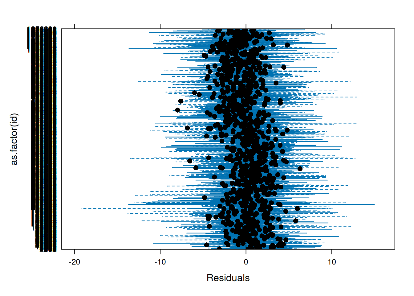
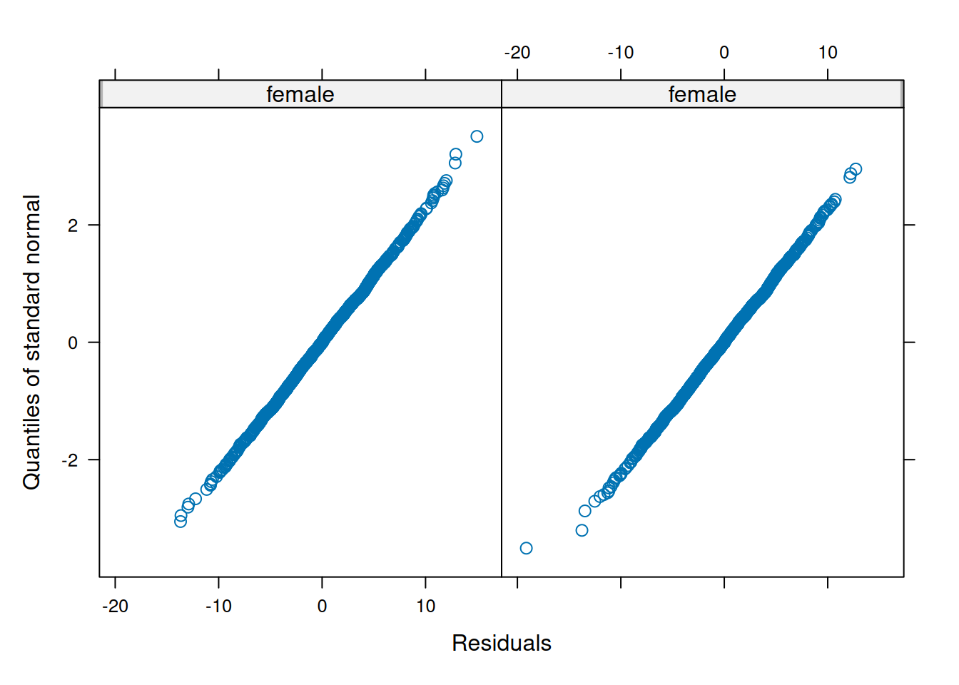
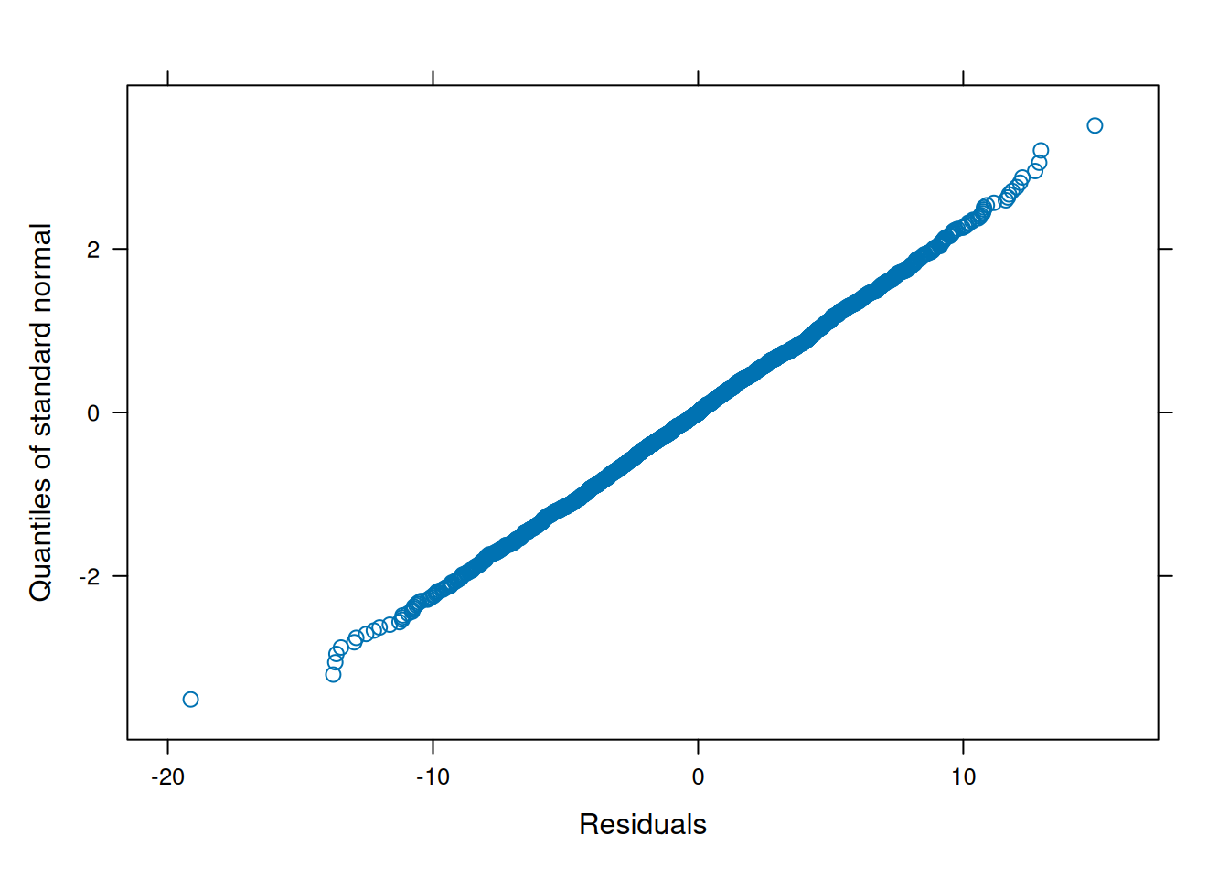
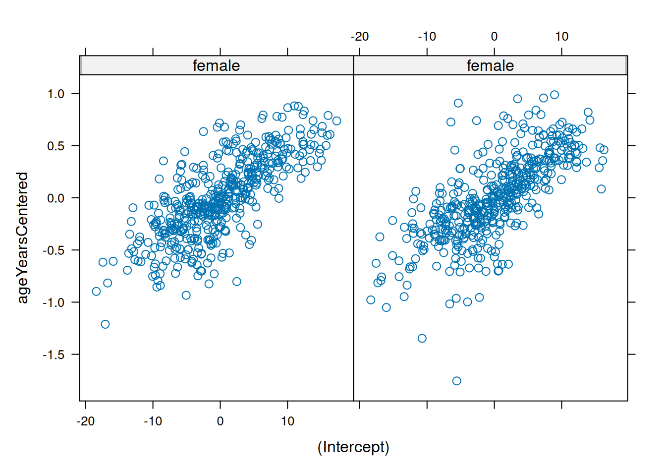
Make QQ plots for each level of the random effects. Vary the level from 0, 1, to 2 so that you can check the between- and within-subject residuals.

qqnorm(
  linearMixedModel_nlme,
  ~ ranef(., level = 1))

16.3 PP Plots

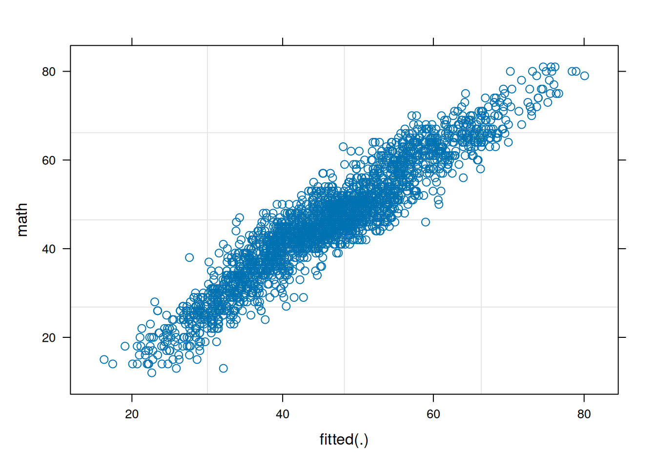
ppPlot(linearMixedModel)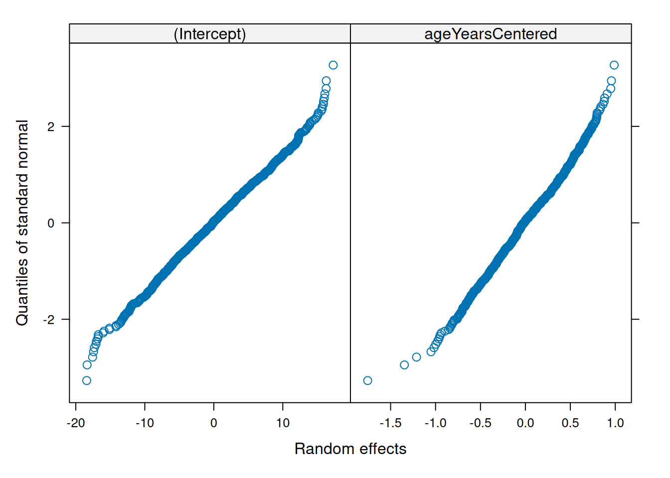

16.4 QQ Plot of residuals

qqnorm(resid(linearMixedModel))
qqline(resid(linearMixedModel))

16.5 Plot residuals

plot(linearMixedModel)

16.6 Plot residuals by group (in the example below, level 2 represents the individual)

plot(
  linearMixedModel,
  as.factor(id) ~ resid(.),
  abline = 0,
  xlab = "Residuals")

16.7 Plot residuals by levels of a predictor

plot(
  linearMixedModel_nlme,
  resid(., type = "p") ~ fitted(.) | female) #type = "p" specifies standardized residuals

16.8 Can model heteroscedasticity of the within-group error with the weights argument

linearMixedModel_nlmeVarStructure <- lme(
  math ~ female + ageYearsCentered,
  random = ~ 1 + ageYearsCentered|id,
  weights = varIdent(form = ~ 1 | female),
  method = "ML",
  data = mydata,
  na.action = na.exclude)

summary(linearMixedModel_nlmeVarStructure)

Linear mixed-effects model fit by maximum likelihood
  Data: mydata 
       AIC      BIC    logLik
  15857.83 15903.48 -7920.915

Random effects:
 Formula: ~1 + ageYearsCentered | id
 Structure: General positive-definite, Log-Cholesky parametrization
                 StdDev    Corr  
(Intercept)      7.9177716 (Intr)
ageYearsCentered 0.8278343 0.076 
Residual         5.6410162       

Variance function:
 Structure: Different standard deviations per stratum
 Formula: ~1 | female 
 Parameter estimates:
       1        0 
1.000000 1.009161 
Fixed effects:  math ~ female + ageYearsCentered 
                     Value Std.Error   DF  t-value p-value
(Intercept)      30.554856 0.5040373 1288 60.62022  0.0000
female           -0.692653 0.6172485  930 -1.12216  0.2621
ageYearsCentered  4.255258 0.0805531 1288 52.82553  0.0000
 Correlation: 
                 (Intr) female
female           -0.614       
ageYearsCentered -0.507  0.014

Standardized Within-Group Residuals:
        Min          Q1         Med          Q3         Max 
-3.37982974 -0.51663213  0.00445497  0.52228733  2.63205084 

Number of Observations: 2221
Number of Groups: 932 

16.9 Plot observed and fitted values

plot(
  linearMixedModel,
  math ~ fitted(.))

16.10 Plot QQ plot of residuals by levels of a predictor

qqnorm(linearMixedModel_nlme, ~ resid(.) | female)

qqnorm(linearMixedModel_nlme, ~ resid(.))

16.11 QQ plot of random effects

Make QQ plots for each level of the random effects. Vary the level from 0, 1, to 2 so that you can check the between- and within-subject residuals.

qqnorm(
  linearMixedModel_nlme,
  ~ ranef(., level = 0))

Error in `effects[[1L]]`:
! subscript out of bounds

qqnorm(
  linearMixedModel_nlme,
  ~ ranef(., level = 1))

qqnorm(
  linearMixedModel_nlme,
  ~ ranef(., level = 2))

Error:
! object '.y' not found

16.12 QQ plot of random effects by levels of a predictor

qqnorm(
  linearMixedModel_nlme,
  ~ ranef(., level = 1) | female)

16.13 Pairs plot

pairs(linearMixedModel_nlme)

pairs(
  linearMixedModel_nlme,
  ~ ranef(., level = 1) | female)

16.14 Variance functions for modeling heteroscedasticity

• varFixed: fixed variance
• varIdent: different variances per stratum
• varPower: power of covariate
• varExp: exponential of covariate
• varConstPower: constant plus power of covariate
• varComb: combination of variance functions

16.15 Correlation structures for modeling dependence

• corCompSymm: compound symmetry
• corSymm: general
• corAR1: autoregressive of order 1
• corCAR1: continuous-time AR(1)
• corARMA: autoregressive-moving average
• corExp: exponential
• corGaus: Gaussian
• corLin: linear
• corRatio: rational quadratic
• corSpher: spherical

17 Power Analysis

• mlmpower: https://github.com/bkeller2/mlmpower (Enders et al., 2025)
• https://aguinis.shinyapps.io/ml_power/
• https://www.causalevaluation.org/power-analysis.html
  • https://powerupr.shinyapps.io/index/
• https://koumurayama.shinyapps.io/tmethod_mlm/
• https://webpower.psychstat.org/wiki/models/index

18 Session Info

sessionInfo()

R version 4.6.1 (2026-06-24)
Platform: x86_64-pc-linux-gnu
Running under: Ubuntu 24.04.4 LTS

Matrix products: default
BLAS:   /usr/lib/x86_64-linux-gnu/openblas-pthread/libblas.so.3 
LAPACK: /usr/lib/x86_64-linux-gnu/openblas-pthread/libopenblasp-r0.3.26.so;  LAPACK version 3.12.0

locale:
 [1] LC_CTYPE=C.UTF-8       LC_NUMERIC=C           LC_TIME=C.UTF-8       
 [4] LC_COLLATE=C.UTF-8     LC_MONETARY=C.UTF-8    LC_MESSAGES=C.UTF-8   
 [7] LC_PAPER=C.UTF-8       LC_NAME=C              LC_ADDRESS=C          
[10] LC_TELEPHONE=C         LC_MEASUREMENT=C.UTF-8 LC_IDENTIFICATION=C   

time zone: UTC
tzcode source: system (glibc)

attached base packages:
[1] stats     graphics  grDevices utils     datasets  methods   base     

other attached packages:
 [1] lubridate_1.9.5    forcats_1.0.1      stringr_1.6.0      dplyr_1.2.1       
 [5] purrr_1.2.2        readr_2.2.0        tidyr_1.3.2        tibble_3.3.1      
 [9] tidyverse_2.0.0    ggforce_0.5.0      ggplot2_4.0.3      performance_0.17.1
[13] parallelly_1.48.0  mgcv_1.9-4         MCMCglmm_2.36      ape_5.8-1         
[17] coda_0.19-4.1      MASS_7.3-65        lmerTest_3.2-1     nlme_3.1-169      
[21] lme4_2.0-6         Matrix_1.7-5       petersenlab_1.2.3 

loaded via a namespace (and not attached):
 [1] Rdpack_2.6.6        DBI_1.3.0           mnormt_2.1.2       
 [4] gridExtra_2.3.1     rlang_1.3.0         magrittr_2.0.5     
 [7] otel_0.2.0          compiler_4.6.1      vctrs_0.7.3        
[10] reshape2_1.4.5      quadprog_1.5-8      pkgconfig_2.0.3    
[13] fastmap_1.2.0       backports_1.5.1     labeling_0.4.3     
[16] pbivnorm_0.6.0      effectsize_1.0.3    rmarkdown_2.31     
[19] tzdb_0.5.0          nloptr_2.2.1        xfun_0.60          
[22] jsonlite_2.0.0      tweenr_2.0.3        psych_2.6.5        
[25] parallel_4.6.1      lavaan_0.7-2        cluster_2.1.8.2    
[28] R6_2.6.1            stringi_1.8.9       RColorBrewer_1.1-3 
[31] boot_1.3-32         rpart_4.1.27        numDeriv_2016.8-1.1
[34] Rcpp_1.1.2          knitr_1.51          parameters_0.29.2  
[37] base64enc_0.1-6     splines_4.6.1       nnet_7.3-20        
[40] timechange_0.4.0    tidyselect_1.2.1    rstudioapi_0.19.0  
[43] yaml_2.3.12         lattice_0.22-9      plyr_1.8.9         
[46] withr_3.0.3         bayestestR_0.18.1   S7_0.2.2           
[49] evaluate_1.0.5      foreign_0.8-91      polyclip_1.10-7    
[52] pillar_1.11.1       tensorA_0.36.2.1    checkmate_2.3.4    
[55] stats4_4.6.1        reformulas_0.4.4    insight_1.5.2      
[58] generics_0.1.4      mix_1.0-13          hms_1.1.4          
[61] scales_1.4.0        minqa_1.2.8         xtable_1.8-8       
[64] glue_1.8.1          cubature_2.1.4-1    Hmisc_5.2-6        
[67] tools_4.6.1         data.table_1.18.4   mvtnorm_1.4-2      
[70] grid_4.6.1          mitools_2.4         rbibutils_2.4.1    
[73] datawizard_1.3.1    colorspace_2.1-3    htmlTable_2.5.0    
[76] Formula_1.2-6       cli_3.6.6           viridisLite_0.4.3  
[79] corpcor_1.6.10      gtable_0.3.6        digest_0.6.39      
[82] htmlwidgets_1.6.4   farver_2.1.2        htmltools_0.5.9    
[85] lifecycle_1.0.5